# (Install and) load pacman package
if (!require(pacman)) install.packages("pacman")

# load packages that are already installed and install packages that are not
# installed yet and then load them:
pacman::p_load(tinylabels,
               papaja,
               haven,
               labelled,
               janitor,
               skimr,
               rstatix,
               HH,
               likert,
               expss,
               tidyr,
               ggstats,
               psych,
               sjlabelled,
               sjmisc,
               tidyverse,
               MASS,
               dplyr,
               magick,
               tinytable)

# sessionInfo()7 Descriptive Statistics of the NRW80+ Dataset
In this chapter, I illustrate the process of importing NRW80+ data (see Zank et al., 2022) into R. Additionally, I present descriptive statistics and graphical visualizations to gain insights into Likert-scaled surveys. The paper adheres to the APA style, implementing the R template provided by the ‘papaja’ package (Aust & Barth, 2023).
Zank, S., Woopen, C., Wagner, M., Rietz, C., & Kaspar, R. (2022). Quality of Life and Well-being of Very Old People in NRW (Representative Survey NRW80+) - Cross-Section Wave 1. GESIS, Cologne. ZA7558 Data file Version 2.0.0. https://doi.org/10.4232/1.13978
Aust, F., & Barth, M. (2023). papaja: Prepare reproducible APA journal articles with R Markdown. https://github.com/crsh/papaja
7.1 Technical Note
In the following, I load (and install) packages that I use later on and I show information about my R session with sessionInfo().
7.2 Import Data
I host a R script on my GitHub account (see https://raw.githubusercontent.com/hubchev/courses/main/scr/readin_GESIS.R) that explains how to import the NRW80+ data. I have manually saved the data, gesis.RData, in a subfolder named data.
7.3 How to Use the NRW80+ Data
7.3.1 Load and Subset Data
I load the data and select some variables that are of particular interest to me.
getwd()[1] "/home/sthu/Dropbox/hsf/courses/ewa"load("/home/sthu/Dropbox/hsf/23-ws/ewa/data/gesis.RData")
df <- dfdta |>
select(starts_with("alter"),
ALT_agegroup,
ALT_sex,
famst1, famst7,
demtectcorr,
kogstat,
final,
geschlecht)
# Remove the common prefix from all variables
df <- df |>
mutate_all(~ set_label(., gsub("^Alternserleben: ", "", get_label(.))))For simplification, let us focus on the questions that refer to the “Experience of Ageing” and create a new dataset df_alterl that contains only those questions:
df_alterl <- df |>
  select(alterl1,
         alterl2,
         alterl3,
         alterl4,
         alterl5,
         alterl6,
         alterl7,
         alterl8,
         alterl9,
         alterl10) |>
  drop_unused_labels()

# to remove unused labels you can use drop_unused_labels():
df_alterl_un <- df_alterl |>
  drop_unused_labels()

summary(df_alterl)
alterl1 alterl2 alterl3 alterl4
Min. :-2.000 Min. :-2.000 Min. :-2.000 Min. :-2.000
1st Qu.: 1.000 1st Qu.: 2.000 1st Qu.: 1.000 1st Qu.: 2.000
Median : 3.000 Median : 4.000 Median : 2.000 Median : 3.000
Mean : 2.656 Mean : 3.282 Mean : 2.349 Mean : 2.763
3rd Qu.: 4.000 3rd Qu.: 4.000 3rd Qu.: 3.000 3rd Qu.: 4.000
Max. : 5.000 Max. : 5.000 Max. : 5.000 Max. : 5.000
alterl5 alterl6 alterl7 alterl8
Min. :-2.00 Min. :-2.000 Min. :-2.000 Min. :-2.000
1st Qu.: 2.00 1st Qu.: 2.000 1st Qu.: 2.000 1st Qu.: 1.000
Median : 3.00 Median : 4.000 Median : 3.000 Median : 3.000
Mean : 2.99 Mean : 3.405 Mean : 3.237 Mean : 2.712
3rd Qu.: 4.00 3rd Qu.: 5.000 3rd Qu.: 4.000 3rd Qu.: 4.000
Max. : 5.00 Max. : 5.000 Max. : 5.000 Max. : 5.000
alterl9 alterl10
Min. :-2.000 Min. :-2.000
1st Qu.: 2.000 1st Qu.: 1.000
Median : 3.000 Median : 2.000
Mean : 2.969 Mean : 2.305
3rd Qu.: 4.000 3rd Qu.: 3.000
Max. : 5.000 Max. : 5.000 7.3.2 Get an Overview by Counting
7.3.2.1 table() of R base
With the table() function, you can count how many observations of each unique value a variable contains:
table(df_alterl$alterl1)
Weiß nicht Verweigert  Gar nicht  Ein wenig      Mäßig      Stark Sehr stark
        80          6        390        266        451        511        159
To do that for each variable of a dataset is easy using ~, the pipe operator, and map() of the package purrr (Wickham & Henry, 2023):
Wickham, H., & Henry, L. (2023). purrr: Functional Programming Tools. https://CRAN.R-project.org/package=purrr
df_alterl |>
  map(~ table(.))
$alterl1
.
Weiß nicht Verweigert Gar nicht Ein wenig Mäßig Stark Sehr stark
80 6 390 266 451 511 159
$alterl2
.
Weiß nicht Verweigert Gar nicht Ein wenig Mäßig Stark Sehr stark
36 4 196 245 379 648 355
$alterl3
.
Weiß nicht Verweigert Gar nicht Ein wenig Mäßig Stark Sehr stark
20 3 500 577 403 244 116
$alterl4
.
Weiß nicht Verweigert Gar nicht Ein wenig Mäßig Stark Sehr stark
122 8 222 260 527 543 181
$alterl5
.
Weiß nicht Verweigert Gar nicht Ein wenig Mäßig Stark Sehr stark
101 4 199 211 452 680 216
$alterl6
.
Weiß nicht Verweigert Gar nicht Ein wenig Mäßig Stark Sehr stark
19 3 149 324 358 537 473
$alterl7
.
Weiß nicht Verweigert Gar nicht Ein wenig Mäßig Stark Sehr stark
20 2 145 362 471 525 338
$alterl8
.
Weiß nicht Verweigert Gar nicht Ein wenig Mäßig Stark Sehr stark
20 3 516 350 325 340 309
$alterl9
.
Weiß nicht Verweigert Gar nicht Ein wenig Mäßig Stark Sehr stark
83 10 261 228 425 564 292
$alterl10
.
Weiß nicht Verweigert Gar nicht Ein wenig Mäßig Stark Sehr stark
44 7 537 433 486 251 105 Using proportions() returns the conditional proportions:
df_alterl |>
  map(~ proportions(table(.)))
$alterl1
.
Weiß nicht Verweigert Gar nicht Ein wenig Mäßig Stark
0.042941492 0.003220612 0.209339775 0.142780462 0.242082662 0.274288782
Sehr stark
0.085346216
$alterl2
.
Weiß nicht Verweigert Gar nicht Ein wenig Mäßig Stark
0.019323671 0.002147075 0.105206656 0.131508320 0.203435319 0.347826087
Sehr stark
0.190552872
$alterl3
.
Weiß nicht Verweigert Gar nicht Ein wenig Mäßig Stark
0.010735373 0.001610306 0.268384326 0.309715513 0.216317767 0.130971551
Sehr stark
0.062265164
$alterl4
.
Weiß nicht Verweigert Gar nicht Ein wenig Mäßig Stark
0.065485776 0.004294149 0.119162641 0.139559850 0.282877080 0.291465378
Sehr stark
0.097155126
$alterl5
.
Weiß nicht Verweigert Gar nicht Ein wenig Mäßig Stark
0.054213634 0.002147075 0.106816962 0.113258186 0.242619431 0.365002684
Sehr stark
0.115942029
$alterl6
.
Weiß nicht Verweigert Gar nicht Ein wenig Mäßig Stark
0.010198604 0.001610306 0.079978529 0.173913043 0.192163178 0.288244767
Sehr stark
0.253891573
$alterl7
.
Weiß nicht Verweigert Gar nicht Ein wenig Mäßig Stark
0.010735373 0.001073537 0.077831455 0.194310252 0.252818035 0.281803543
Sehr stark
0.181427805
$alterl8
.
Weiß nicht Verweigert Gar nicht Ein wenig Mäßig Stark
0.010735373 0.001610306 0.276972625 0.187869028 0.174449812 0.182501342
Sehr stark
0.165861514
$alterl9
.
Weiß nicht Verweigert Gar nicht Ein wenig Mäßig Stark
0.044551798 0.005367687 0.140096618 0.122383253 0.228126677 0.302737520
Sehr stark
0.156736447
$alterl10
.
Weiß nicht Verweigert Gar nicht Ein wenig Mäßig Stark
0.023617821 0.003757381 0.288244767 0.232420827 0.260869565 0.134728932
Sehr stark
0.056360709 7.3.2.2 tabyl() of janitor
With tabyl() which is part of janitor (Firke, 2023), we can get both nicely:
Firke, S. (2023). janitor: Simple Tools for Examining and Cleaning Dirty Data. https://CRAN.R-project.org/package=janitor
df_alterl |>
  tabyl(alterl1)
alterl1 n percent
-2 80 0.042941492
-1 6 0.003220612
1 390 0.209339775
2 266 0.142780462
3 451 0.242082662
4 511 0.274288782
5 159 0.085346216df_alterl |>
map(~ tabyl(.))$alterl1
. n percent
-2 80 0.042941492
-1 6 0.003220612
1 390 0.209339775
2 266 0.142780462
3 451 0.242082662
4 511 0.274288782
5 159 0.085346216
$alterl2
. n percent
-2 36 0.019323671
-1 4 0.002147075
1 196 0.105206656
2 245 0.131508320
3 379 0.203435319
4 648 0.347826087
5 355 0.190552872
$alterl3
. n percent
-2 20 0.010735373
-1 3 0.001610306
1 500 0.268384326
2 577 0.309715513
3 403 0.216317767
4 244 0.130971551
5 116 0.062265164
$alterl4
. n percent
-2 122 0.065485776
-1 8 0.004294149
1 222 0.119162641
2 260 0.139559850
3 527 0.282877080
4 543 0.291465378
5 181 0.097155126
$alterl5
. n percent
-2 101 0.054213634
-1 4 0.002147075
1 199 0.106816962
2 211 0.113258186
3 452 0.242619431
4 680 0.365002684
5 216 0.115942029
$alterl6
. n percent
-2 19 0.010198604
-1 3 0.001610306
1 149 0.079978529
2 324 0.173913043
3 358 0.192163178
4 537 0.288244767
5 473 0.253891573
$alterl7
. n percent
-2 20 0.010735373
-1 2 0.001073537
1 145 0.077831455
2 362 0.194310252
3 471 0.252818035
4 525 0.281803543
5 338 0.181427805
$alterl8
. n percent
-2 20 0.010735373
-1 3 0.001610306
1 516 0.276972625
2 350 0.187869028
3 325 0.174449812
4 340 0.182501342
5 309 0.165861514
$alterl9
. n percent
-2 83 0.044551798
-1 10 0.005367687
1 261 0.140096618
2 228 0.122383253
3 425 0.228126677
4 564 0.302737520
5 292 0.156736447
$alterl10
. n percent
-2 44 0.023617821
-1 7 0.003757381
1 537 0.288244767
2 433 0.232420827
3 486 0.260869565
4 251 0.134728932
5 105 0.0563607097.3.2.3 frq() of sjmisc
As the variables df_alterl1 are factors. Thus, we can use the sjmisc package, see Lüdecke (2018) and the cheatsheet of sjmisc http://strengejacke.de/sjmisc-cheatsheet.pdf. Also worth a reading is browseVignettes("sjmisc").
Lüdecke, D. (2018). sjmisc: Data and Variable Transformation Functions. Journal of Open Source Software, 3(26), 754. https://doi.org/10.21105/joss.00754
For example, we can use frq() for nice frequency tables:
df_alterl |>
  map(~ frq(. , show.na = T))
$alterl1
Beziehungen und andere Menschen mehr schätzen (x) <numeric>
# total N=1863 valid N=1863 mean=2.66 sd=1.61
Value | Label | N | Raw % | Valid % | Cum. %
---------------------------------------------------
-2 | Weiß nicht | 0 | 0.00 | 0.00 | 0.00
-1 | Verweigert | 0 | 0.00 | 0.00 | 0.00
1 | Gar nicht | 80 | 4.29 | 4.29 | 4.29
2 | Ein wenig | 6 | 0.32 | 0.32 | 4.62
3 | Mäßig | 390 | 20.93 | 20.93 | 25.55
4 | Stark | 266 | 14.28 | 14.28 | 39.83
5 | Sehr stark | 451 | 24.21 | 24.21 | 64.04
6 | <NA> | 511 | 27.43 | 27.43 | 91.47
7 | <NA> | 159 | 8.53 | 8.53 | 100.00
<NA> | <NA> | 0 | 0.00 | <NA> | <NA>
$alterl2
Gesundheit mehr Aufmerksamkeit widmen (x) <numeric>
# total N=1863 valid N=1863 mean=3.28 sd=1.45
Value | Label | N | Raw % | Valid % | Cum. %
---------------------------------------------------
-2 | Weiß nicht | 0 | 0.00 | 0.00 | 0.00
-1 | Verweigert | 0 | 0.00 | 0.00 | 0.00
1 | Gar nicht | 36 | 1.93 | 1.93 | 1.93
2 | Ein wenig | 4 | 0.21 | 0.21 | 2.15
3 | Mäßig | 196 | 10.52 | 10.52 | 12.67
4 | Stark | 245 | 13.15 | 13.15 | 25.82
5 | Sehr stark | 379 | 20.34 | 20.34 | 46.16
6 | <NA> | 648 | 34.78 | 34.78 | 80.94
7 | <NA> | 355 | 19.06 | 19.06 | 100.00
<NA> | <NA> | 0 | 0.00 | <NA> | <NA>
$alterl3
geistige Leistungsfähigkeit nimmt ab (x) <numeric>
# total N=1863 valid N=1863 mean=2.35 sd=1.28
Value | Label | N | Raw % | Valid % | Cum. %
---------------------------------------------------
-2 | Weiß nicht | 0 | 0.00 | 0.00 | 0.00
-1 | Verweigert | 0 | 0.00 | 0.00 | 0.00
1 | Gar nicht | 20 | 1.07 | 1.07 | 1.07
2 | Ein wenig | 3 | 0.16 | 0.16 | 1.23
3 | Mäßig | 500 | 26.84 | 26.84 | 28.07
4 | Stark | 577 | 30.97 | 30.97 | 59.04
5 | Sehr stark | 403 | 21.63 | 21.63 | 80.68
6 | <NA> | 244 | 13.10 | 13.10 | 93.77
7 | <NA> | 116 | 6.23 | 6.23 | 100.00
<NA> | <NA> | 0 | 0.00 | <NA> | <NA>
$alterl4
mehr Erfahrung, um Dinge und Menschen einzuschätzen (x) <numeric>
# total N=1863 valid N=1863 mean=2.76 sd=1.72
Value | Label | N | Raw % | Valid % | Cum. %
---------------------------------------------------
-2 | Weiß nicht | 0 | 0.00 | 0.00 | 0.00
-1 | Verweigert | 0 | 0.00 | 0.00 | 0.00
1 | Gar nicht | 122 | 6.55 | 6.55 | 6.55
2 | Ein wenig | 8 | 0.43 | 0.43 | 6.98
3 | Mäßig | 222 | 11.92 | 11.92 | 18.89
4 | Stark | 260 | 13.96 | 13.96 | 32.85
5 | Sehr stark | 527 | 28.29 | 28.29 | 61.14
6 | <NA> | 543 | 29.15 | 29.15 | 90.28
7 | <NA> | 181 | 9.72 | 9.72 | 100.00
<NA> | <NA> | 0 | 0.00 | <NA> | <NA>
$alterl5
besseres Gespür, was wichtig ist (x) <numeric>
# total N=1863 valid N=1863 mean=2.99 sd=1.66
Value | Label | N | Raw % | Valid % | Cum. %
---------------------------------------------------
-2 | Weiß nicht | 0 | 0.00 | 0.00 | 0.00
-1 | Verweigert | 0 | 0.00 | 0.00 | 0.00
1 | Gar nicht | 101 | 5.42 | 5.42 | 5.42
2 | Ein wenig | 4 | 0.21 | 0.21 | 5.64
3 | Mäßig | 199 | 10.68 | 10.68 | 16.32
4 | Stark | 211 | 11.33 | 11.33 | 27.64
5 | Sehr stark | 452 | 24.26 | 24.26 | 51.91
6 | <NA> | 680 | 36.50 | 36.50 | 88.41
7 | <NA> | 216 | 11.59 | 11.59 | 100.00
<NA> | <NA> | 0 | 0.00 | <NA> | <NA>
$alterl6
Einschränkung der Aktivitäten (x) <numeric>
# total N=1863 valid N=1863 mean=3.40 sd=1.38
Value | Label | N | Raw % | Valid % | Cum. %
---------------------------------------------------
-2 | Weiß nicht | 0 | 0.00 | 0.00 | 0.00
-1 | Verweigert | 0 | 0.00 | 0.00 | 0.00
1 | Gar nicht | 19 | 1.02 | 1.02 | 1.02
2 | Ein wenig | 3 | 0.16 | 0.16 | 1.18
3 | Mäßig | 149 | 8.00 | 8.00 | 9.18
4 | Stark | 324 | 17.39 | 17.39 | 26.57
5 | Sehr stark | 358 | 19.22 | 19.22 | 45.79
6 | <NA> | 537 | 28.82 | 28.82 | 74.61
7 | <NA> | 473 | 25.39 | 25.39 | 100.00
<NA> | <NA> | 0 | 0.00 | <NA> | <NA>
$alterl7
weniger Energie (x) <numeric>
# total N=1863 valid N=1863 mean=3.24 sd=1.32
Value | Label | N | Raw % | Valid % | Cum. %
---------------------------------------------------
-2 | Weiß nicht | 0 | 0.00 | 0.00 | 0.00
-1 | Verweigert | 0 | 0.00 | 0.00 | 0.00
1 | Gar nicht | 20 | 1.07 | 1.07 | 1.07
2 | Ein wenig | 2 | 0.11 | 0.11 | 1.18
3 | Mäßig | 145 | 7.78 | 7.78 | 8.96
4 | Stark | 362 | 19.43 | 19.43 | 28.40
5 | Sehr stark | 471 | 25.28 | 25.28 | 53.68
6 | <NA> | 525 | 28.18 | 28.18 | 81.86
7 | <NA> | 338 | 18.14 | 18.14 | 100.00
<NA> | <NA> | 0 | 0.00 | <NA> | <NA>
$alterl8
Abhängigkeit von der Hilfe Anderer (x) <numeric>
# total N=1863 valid N=1863 mean=2.71 sd=1.53
Value | Label | N | Raw % | Valid % | Cum. %
---------------------------------------------------
-2 | Weiß nicht | 0 | 0.00 | 0.00 | 0.00
-1 | Verweigert | 0 | 0.00 | 0.00 | 0.00
1 | Gar nicht | 20 | 1.07 | 1.07 | 1.07
2 | Ein wenig | 3 | 0.16 | 0.16 | 1.23
3 | Mäßig | 516 | 27.70 | 27.70 | 28.93
4 | Stark | 350 | 18.79 | 18.79 | 47.72
5 | Sehr stark | 325 | 17.44 | 17.44 | 65.16
6 | <NA> | 340 | 18.25 | 18.25 | 83.41
7 | <NA> | 309 | 16.59 | 16.59 | 100.00
<NA> | <NA> | 0 | 0.00 | <NA> | <NA>
$alterl9
Freiheit, Tage nach eigenem Willen zu verleben (x) <numeric>
# total N=1863 valid N=1863 mean=2.97 sd=1.68
Value | Label | N | Raw % | Valid % | Cum. %
---------------------------------------------------
-2 | Weiß nicht | 0 | 0.00 | 0.00 | 0.00
-1 | Verweigert | 0 | 0.00 | 0.00 | 0.00
1 | Gar nicht | 83 | 4.46 | 4.46 | 4.46
2 | Ein wenig | 10 | 0.54 | 0.54 | 4.99
3 | Mäßig | 261 | 14.01 | 14.01 | 19.00
4 | Stark | 228 | 12.24 | 12.24 | 31.24
5 | Sehr stark | 425 | 22.81 | 22.81 | 54.05
6 | <NA> | 564 | 30.27 | 30.27 | 84.33
7 | <NA> | 292 | 15.67 | 15.67 | 100.00
<NA> | <NA> | 0 | 0.00 | <NA> | <NA>
$alterl10
Motivation fällt schwerer (x) <numeric>
# total N=1863 valid N=1863 mean=2.31 sd=1.38
Value | Label | N | Raw % | Valid % | Cum. %
---------------------------------------------------
-2 | Weiß nicht | 0 | 0.00 | 0.00 | 0.00
-1 | Verweigert | 0 | 0.00 | 0.00 | 0.00
1 | Gar nicht | 44 | 2.36 | 2.36 | 2.36
2 | Ein wenig | 7 | 0.38 | 0.38 | 2.74
3 | Mäßig | 537 | 28.82 | 28.82 | 31.56
4 | Stark | 433 | 23.24 | 23.24 | 54.80
5 | Sehr stark | 486 | 26.09 | 26.09 | 80.89
6 | <NA> | 251 | 13.47 | 13.47 | 94.36
7 | <NA> | 105 | 5.64 | 5.64 | 100.00
<NA> | <NA> | 0 | 0.00 | <NA> | <NA>7.3.3 First Summary Statistics
7.3.3.1 Using summary() and get_summary_stats()
First, I am interested in the class of the data and some very basic summary statistics.
summary(df) alterl1 alterl2 alterl3 alterl4
Min. :-2.000 Min. :-2.000 Min. :-2.000 Min. :-2.000
1st Qu.: 1.000 1st Qu.: 2.000 1st Qu.: 1.000 1st Qu.: 2.000
Median : 3.000 Median : 4.000 Median : 2.000 Median : 3.000
Mean : 2.656 Mean : 3.282 Mean : 2.349 Mean : 2.763
3rd Qu.: 4.000 3rd Qu.: 4.000 3rd Qu.: 3.000 3rd Qu.: 4.000
Max. : 5.000 Max. : 5.000 Max. : 5.000 Max. : 5.000
alterl5 alterl6 alterl7 alterl8
Min. :-2.00 Min. :-2.000 Min. :-2.000 Min. :-2.000
1st Qu.: 2.00 1st Qu.: 2.000 1st Qu.: 2.000 1st Qu.: 1.000
Median : 3.00 Median : 4.000 Median : 3.000 Median : 3.000
Mean : 2.99 Mean : 3.405 Mean : 3.237 Mean : 2.712
3rd Qu.: 4.00 3rd Qu.: 5.000 3rd Qu.: 4.000 3rd Qu.: 4.000
Max. : 5.00 Max. : 5.000 Max. : 5.000 Max. : 5.000
alterl9 alterl10 alter_int alter_cont
Min. :-2.000 Min. :-2.000 Min. : 80.00 Min. : 80.11
1st Qu.: 2.000 1st Qu.: 1.000 1st Qu.: 82.00 1st Qu.: 82.99
Median : 3.000 Median : 2.000 Median : 86.00 Median : 86.59
Mean : 2.969 Mean : 2.305 Mean : 86.48 Mean : 86.98
3rd Qu.: 4.000 3rd Qu.: 3.000 3rd Qu.: 90.00 3rd Qu.: 90.56
Max. : 5.000 Max. : 5.000 Max. :102.00 Max. :102.92
NA's :6 NA's :6
alterl_m1 alterl_m2 alterp ALT_agegroup
Min. :1.000 Min. :1.000 Min. :-4.000 Min. :1.000
1st Qu.:2.600 1st Qu.:2.200 1st Qu.:-4.000 1st Qu.:1.000
Median :3.200 Median :2.800 Median :-4.000 Median :2.000
Mean :3.168 Mean :2.877 Mean : 2.632 Mean :1.883
3rd Qu.:3.800 3rd Qu.:3.600 3rd Qu.:-4.000 3rd Qu.:3.000
Max. :5.000 Max. :5.000 Max. :99.000 Max. :3.000
NA's :16 NA's :14
ALT_sex famst1 famst7 demtectcorr
Min. :1.000 Min. :-1.000 Min. :-3.000 Min. :-11.000
1st Qu.:1.000 1st Qu.: 1.000 1st Qu.:-3.000 1st Qu.: -1.000
Median :2.000 Median : 4.000 Median : 0.000 Median : 0.000
Mean :1.502 Mean : 2.765 Mean :-1.179 Mean : -1.742
3rd Qu.:2.000 3rd Qu.: 4.000 3rd Qu.: 0.000 3rd Qu.: 0.000
Max. :2.000 Max. : 5.000 Max. : 1.000 Max. : 2.000
kogstat final geschlecht
Min. :-4.00 Min. :81.00 Min. :1.000
1st Qu.:-4.00 1st Qu.:81.00 1st Qu.:1.000
Median :-4.00 Median :81.00 Median :2.000
Mean :-3.21 Mean :81.09 Mean :1.502
3rd Qu.:-4.00 3rd Qu.:81.00 3rd Qu.:2.000
Max. : 7.00 Max. :82.00 Max. :2.000
sumstat_alter <- df |>
  get_summary_stats(
    alterl1,
    alterl2,
    alterl3,
    alterl4,
    alterl5,
    alterl6,
    alterl7,
    alterl8,
    alterl9,
    alterl10,
    type = "five_number")
Warning: attributes are not identical across measure variables; they will be
droppedsumstat_alter# A tibble: 10 × 7
variable n min max q1 median q3
<fct> <dbl> <dbl> <dbl> <dbl> <dbl> <dbl>
1 alterl1 1863 -2 5 1 3 4
2 alterl2 1863 -2 5 2 4 4
3 alterl3 1863 -2 5 1 2 3
4 alterl4 1863 -2 5 2 3 4
5 alterl5 1863 -2 5 2 3 4
6 alterl6 1863 -2 5 2 4 5
7 alterl7 1863 -2 5 2 3 4
8 alterl8 1863 -2 5 1 3 4
9 alterl9 1863 -2 5 2 3 4
10 alterl10 1863 -2 5 1 2 37.3.3.2 Using psych::describe()
A powerful alternative for descriptive summary statistics is provided by the function describe() of the psych package (William Revelle, 2023).
sumstat_alter_psych <- df |>
  select(starts_with("alterl")) |>
  select(-ends_with("m1"), -ends_with("m2")) |>
  psych::describe() |>
  as_tibble(rownames="Question")  |>
  select(-skew, -kurtosis, -range, -vars)

sumstat_alter_psych
# A tibble: 10 × 10
Question n mean sd median trimmed mad min max se
<chr> <dbl> <dbl> <dbl> <dbl> <dbl> <dbl> <dbl> <dbl> <dbl>
1 alterl1 1863 2.66 1.61 3 2.76 1.48 -2 5 0.0374
2 alterl2 1863 3.28 1.45 4 3.43 1.48 -2 5 0.0336
3 alterl3 1863 2.35 1.28 2 2.28 1.48 -2 5 0.0296
4 alterl4 1863 2.76 1.72 3 2.96 1.48 -2 5 0.0398
5 alterl5 1863 2.99 1.66 3 3.20 1.48 -2 5 0.0385
6 alterl6 1863 3.40 1.38 4 3.54 1.48 -2 5 0.0321
7 alterl7 1863 3.24 1.32 3 3.33 1.48 -2 5 0.0306
8 alterl8 1863 2.71 1.53 3 2.68 1.48 -2 5 0.0355
9 alterl9 1863 2.97 1.68 3 3.14 1.48 -2 5 0.0389
10 alterl10 1863 2.31 1.38 2 2.28 1.48 -2 5 0.03217.3.3.3 Using summarize() and the tidyverse
As you may be aware, the tidyverse package provides powerful and flexible functions such as filter, select, group_by, and summarize. Here is an example demonstrating how these functions can be utilized to create descriptive statistic tables:
descriptives <- dfdta |>
  # filter(alterl1 > 0) |>
  group_by(geschlecht)  |>
  summarize(
    Mean = mean(alterl1)
    , Count = n()
    , SD = sd(alterl1)
    , Min = min(alterl1)
    , Max = max(alterl1)
  )

descriptives
# A tibble: 2 × 6
geschlecht Mean Count SD Min Max
<dbl+lbl> <dbl> <int> <dbl> <dbl+lbl> <dbl+lbl>
1 1 [Männlich] 2.71 927 1.50 -2 [Weiß nicht] 5 [Sehr stark]
2 2 [Weiblich] 2.60 936 1.72 -2 [Weiß nicht] 5 [Sehr stark]7.3.4 Make Tables using tt()
```{r, echo=FALSE, eval=TRUE, message=FALSE, warning=FALSE}
#| label: tbl-tabrstatix
#| tbl-cap: "Summary Statistics: Experience of Ageing."

tt(sumstat_alter,  output = "markdown",
   note = "Note: This table contains all variables of `alterl*`.")
```| variable | n | min | max | q1 | median | q3 |
|---|---|---|---|---|---|---|
| Note: This table contains all variables of `alterl*`. | ||||||
| alterl1 | 1863 | -2 | 5 | 1 | 3 | 4 |
| alterl2 | 1863 | -2 | 5 | 2 | 4 | 4 |
| alterl3 | 1863 | -2 | 5 | 1 | 2 | 3 |
| alterl4 | 1863 | -2 | 5 | 2 | 3 | 4 |
| alterl5 | 1863 | -2 | 5 | 2 | 3 | 4 |
| alterl6 | 1863 | -2 | 5 | 2 | 4 | 5 |
| alterl7 | 1863 | -2 | 5 | 2 | 3 | 4 |
| alterl8 | 1863 | -2 | 5 | 1 | 3 | 4 |
| alterl9 | 1863 | -2 | 5 | 2 | 3 | 4 |
| alterl10 | 1863 | -2 | 5 | 1 | 2 | 3 |
```{r, echo=FALSE, eval=TRUE, message=FALSE, warning=FALSE}
#| label: tbl-tabsumstatalterpsych
#| tbl-cap: "Summary Statistics: Experience of Ageing (psych)"

tt(sumstat_alter,  output = "markdown",
   note = "Note: This table contains all variables of `alterl*`.")
```| variable | n | min | max | q1 | median | q3 |
|---|---|---|---|---|---|---|
| Note: This table contains all variables of `alterl*`. | ||||||
| alterl1 | 1863 | -2 | 5 | 1 | 3 | 4 |
| alterl2 | 1863 | -2 | 5 | 2 | 4 | 4 |
| alterl3 | 1863 | -2 | 5 | 1 | 2 | 3 |
| alterl4 | 1863 | -2 | 5 | 2 | 3 | 4 |
| alterl5 | 1863 | -2 | 5 | 2 | 3 | 4 |
| alterl6 | 1863 | -2 | 5 | 2 | 4 | 5 |
| alterl7 | 1863 | -2 | 5 | 2 | 3 | 4 |
| alterl8 | 1863 | -2 | 5 | 1 | 3 | 4 |
| alterl9 | 1863 | -2 | 5 | 2 | 3 | 4 |
| alterl10 | 1863 | -2 | 5 | 1 | 2 | 3 |
```{r, echo=FALSE, eval=TRUE, message=FALSE, warning=FALSE}
#| label: tbl-tabsumstatalterpsychbal
#| tbl-cap: "Summary Statistics: Experience of Ageing (psych)"

tt(sumstat_alter_psych, output = "markdown",
  note = "This table contains all variables of `alterl*` and only observations where all questions had been answered.")
```| Question | n | mean | sd | median | trimmed | mad | min | max | se |
|---|---|---|---|---|---|---|---|---|---|
| alterl1 | 1863 | 2.655931 | 1.613659 | 3 | 2.757210 | 1.4826 | -2 | 5 | 0.03738568 |
| alterl2 | 1863 | 3.281804 | 1.449666 | 4 | 3.429913 | 1.4826 | -2 | 5 | 0.03358626 |
| alterl3 | 1863 | 2.348900 | 1.278429 | 2 | 2.277666 | 1.4826 | -2 | 5 | 0.02961898 |
| alterl4 | 1863 | 2.763285 | 1.716885 | 3 | 2.963783 | 1.4826 | -2 | 5 | 0.03977726 |
| alterl5 | 1863 | 2.990338 | 1.661439 | 3 | 3.196512 | 1.4826 | -2 | 5 | 0.03849266 |
| alterl6 | 1863 | 3.404724 | 1.384050 | 4 | 3.537894 | 1.4826 | -2 | 5 | 0.03206605 |
| alterl7 | 1863 | 3.236715 | 1.320460 | 3 | 3.325956 | 1.4826 | -2 | 5 | 0.03059276 |
| alterl8 | 1863 | 2.712292 | 1.534387 | 3 | 2.684775 | 1.4826 | -2 | 5 | 0.03554909 |
| alterl9 | 1863 | 2.969404 | 1.677112 | 3 | 3.142186 | 1.4826 | -2 | 5 | 0.03885578 |
| alterl10 | 1863 | 2.305421 | 1.383735 | 2 | 2.284373 | 1.4826 | -2 | 5 | 0.03205875 |
```{r, echo=FALSE, eval=TRUE, message=FALSE, warning=FALSE}
#| label: tbl-tabdescriptives
#| tbl-cap: "Experience of Ageing: Valuing Relationships and Other People More (By Gender)"

tt(descriptives, output = "markdown")
```| geschlecht | Mean | Count | SD | Min | Max |
|---|---|---|---|---|---|
| 1 | 2.713053 | 927 | 1.500062 | -2 | 5 |
| 2 | 2.599359 | 936 | 1.717715 | -2 | 5 |
Table Tabelle 7.1 was created with the function get_summary_stats() of the rstatix package (Kassambara, 2023), Tables Tabelle 7.2 and Tabelle 7.3 were created with the function describe() of the psych package (William Revelle, 2023), and Table Tabelle 7.4 was created with the function summarize() of the dplyr package (Wickham et al., 2023).
Kassambara, A. (2023). rstatix: Pipe-Friendly Framework for Basic Statistical Tests. https://CRAN.R-project.org/package=rstatix
William Revelle. (2023). psych: Procedures for Psychological, Psychometric, and Personality Research. Northwestern University. https://CRAN.R-project.org/package=psych
Wickham, H., François, R., Henry, L., Müller, K., & Vaughan, D. (2023). dplyr: A Grammar of Data Manipulation. https://CRAN.R-project.org/package=dplyr
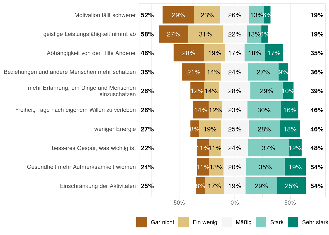
7.3.5 Use the Likert Scale using gglikert()
We have seen that the data contain not only the five different (Likert scaled) answers. Thus, let us remove all values that have, in one or multiple questions, no answer of the Likert scale. The cleaned dataset is named df_alterl_balance.
df_alterl_balance <- df_alterl %>%
rowwise() %>%
mutate(has_negative = ifelse(any(c(across(alterl1:alterl10)) < 0), 1, 0)) |>
filter(has_negative == 0) |>
select(starts_with("alter")) |>
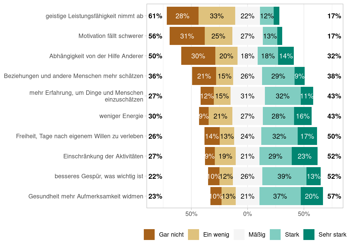
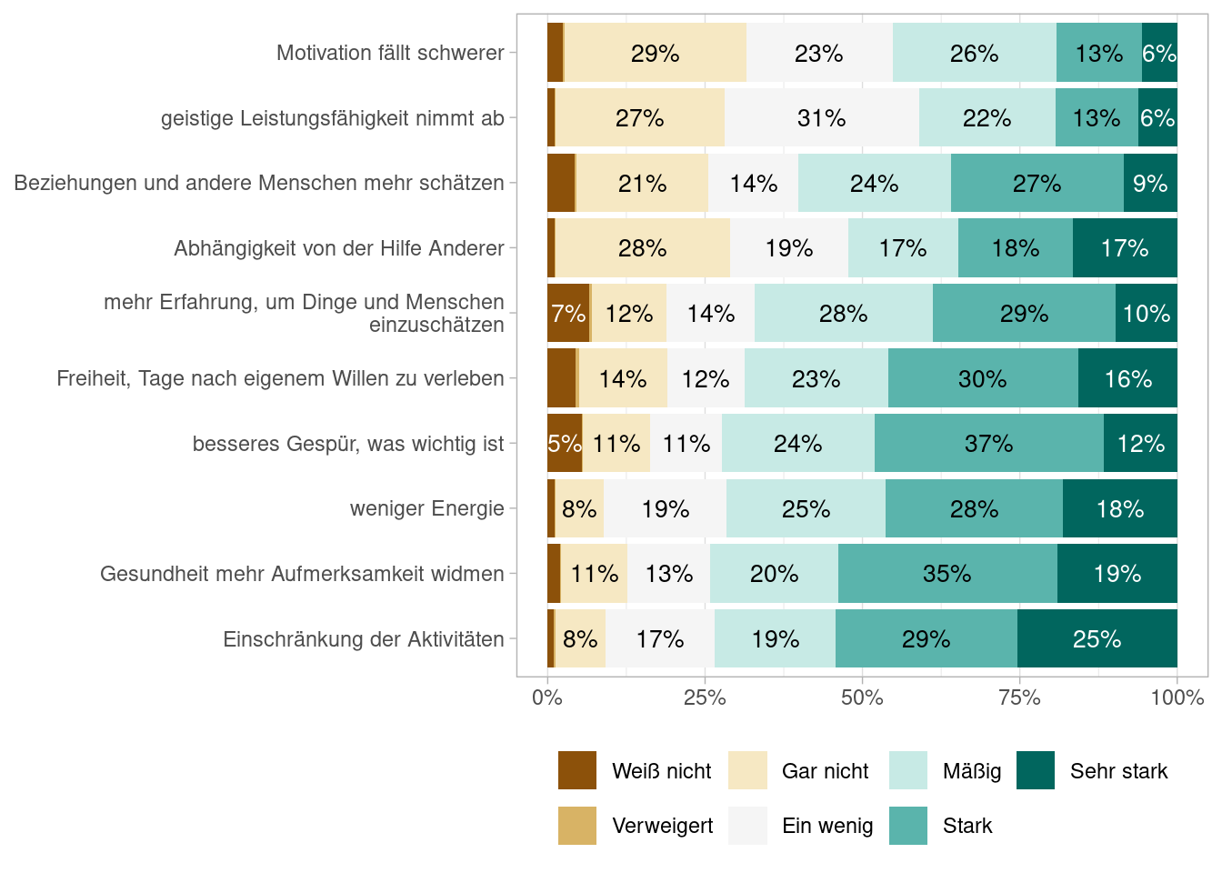
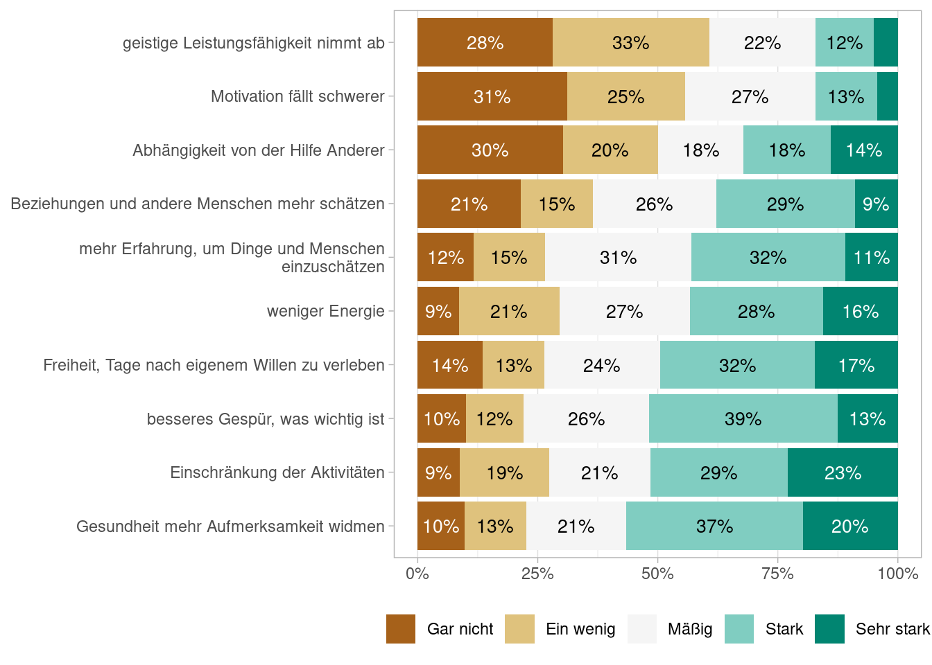
as_tibble()Using the gglikert() of the ggstats package (Larmarange, 2023) allows us to draw nice graphs. I highly recommend reading the vignette of the package in the R documentation which you get with vignette("gglikert").
Larmarange, J. (2023). ggstats: Extension to ’ggplot2’ for Plotting Stats. https://CRAN.R-project.org/package=ggstats
Figures Abbildung 7.1 and Abbildung 7.3 shows the proportions of answers using df_alterl data and Figures Abbildung 7.2 and Abbildung 7.4 does so using the df_alterl_balance data whereby the latter to show the proportions stacked. Do you see any difference and can you explain the differences?
As we are interested in the differences of the two samples, it makes sense to look as the summary statistics for the df_alter_balance sample. This is shown in Table Tabelle 7.3.
7.4 Cross-Referencing in R Markdown
In adherence to the APA style guidelines (Association et al., 2022), it is imperative to reference all figures and tables by their respective numbers within the text. Avoid using generic phrases like “the table above” or “the figure below.” Additionally, refrain from hard-coding the numbers for a more dynamic and standardized approach. Xie et al. (2023) explains concisely how to do that with R Markdown, see: https://bookdown.org/yihui/rmarkdown-cookbook/cross-ref.html.
Association, A. P. et al. (2022). Publication manual of the American psychological association. : American Psychological Association.
Xie, Y., Dervieux, C., & Riederer, E. (2023). R Markdown Cookbook. online. https://bookdown.org/yihui/rmarkdown-cookbook/
For example, I can refer to Table Tabelle 7.1 with @tbl-tabrstatix because I have specified the corresponding label in the R code-chunk, see:
7.5 Exercises
With
knitr::purl("desc_NRW80.Rmd")you can extract the whole R code from the R Markdown file and write it into the R scriptdesc_NRW80.R. Try it.The dataset
gesis.RDatacomes with two different tibbles:dfsavanddfdta. Is there a difference between these two when it comes to the statistics that are shown in this paper? To check that, rename the pdf filedesc_NRW80.pdf, change the code in Section @ref(sec-load) so that you are using the other data (df <- dfdta |> ...vs.df <- dfsav |> ...), knit the Rmd again, and compare the stats.Check possible differences in the
gglikertplots when usingdf_alterl_uninstead ofdf_alterl.The stats above show that dealing with missing or non-standard answers is a crucial thing. Please read chapter Missing Values of Wickham & Grolemund (2023), see: https://r4ds.hadley.nz/missing-values.
The labels of the variables
alterl1:alterl10have “Alternserleben:” at the beginning. This is not necessary and overloads the graphs. Please change the labels for all graphs using the following code in the respective place in the rmd and then knit it again.
Wickham, H., & Grolemund, G. (2023). R for Data Science (2e). https://r4ds.hadley.nz/
# Remove the common prefix from all variables
df <- df |>
  mutate_all(~ set_label(., gsub("^Alternserleben: ", "", get_label(.))))