6 Regression

Please consider my lecture notes concerning Regression Analysis which you find here (Huber, 2024).

Huber, S. (2024). Quantitative Methods: Lecture Notes. https://hubchev.github.io/qm/

Wysocki, A. C., Lawson, K. M., & Rhemtulla, M. (2022). Statistical Control Requires Causal Justification. Advances in Methods and Practices in Psychological Science, 5(2). https://doi.org/10.1177/25152459221095823

Moreover, I highly recommend reading Wysocki et al. (2022) which is freely available here: https://journals.sagepub.com/doi/10.1177/25152459221095823. They explain how difficult it is to use regression analysis to dentify a causal impact. The main insights of the paper are nicely summarized here: https://osf.io/38mxq.

6.1 Making regression tables using `apa_table`

Here is an example how to use apa_table from the papaja package to make regression output tables.

rm(list = ls())

if (!require(pacman)) install.packages("pacman")
pacman::p_load(tidyverse, stargazer, kableExtra, papaja, haven, tinytable)

# Load the mtcars dataset
data("mtcars")

# Fit a linear regression model
m1 <- lm(mpg ~ wt + hp, data = mtcars)
m2 <- lm(mpg ~ wt , data = mtcars)

# Summary of the model
summary(m1)


Call:
lm(formula = mpg ~ wt + hp, data = mtcars)

Residuals:
   Min     1Q Median     3Q    Max 
-3.941 -1.600 -0.182  1.050  5.854 

Coefficients:
            Estimate Std. Error t value Pr(>|t|)    
(Intercept) 37.22727    1.59879  23.285  < 2e-16 ***
wt          -3.87783    0.63273  -6.129 1.12e-06 ***
hp          -0.03177    0.00903  -3.519  0.00145 ** 
---
Signif. codes:  0 '***' 0.001 '**' 0.01 '*' 0.05 '.' 0.1 ' ' 1

Residual standard error: 2.593 on 29 degrees of freedom
Multiple R-squared:  0.8268,    Adjusted R-squared:  0.8148 
F-statistic: 69.21 on 2 and 29 DF,  p-value: 9.109e-12

apa_lm <- apa_print(m1)

```{r  , echo=FALSE, warning=FALSE, message=FALSE}
#| label: tbl-reg_class
#| tbl-cap: Deskriptive Statistiken
#| tbl.align: left

tt(apa_lm$table)
```

Tabelle 6.1: A full regression table.

term	estimate	conf.int	statistic	df	p.value
Intercept	37.23	[33.96, 40.50]	23.28	29	< .001
Wt	-3.88	[-5.17, -2.58]	-6.13	29	< .001
Hp	-0.03	[-0.05, -0.01]	-3.52	29	.001

6.2 Data

In the statistic course of WS 2020, I asked 23 students about their weight, height, sex, and number of siblings:

classdata <- read.csv("https://raw.githubusercontent.com/hubchev/courses/main/dta/classdata.csv")
head(classdata)

  id sex weight height siblings row
1  1   w     53    156        1   g
2  2   w     73    170        1   g
3  3   m     68    169        1   g
4  4   w     67    166        1   g
5  5   w     65    175        1   g
6  6   w     48    161        0   g

6.3 First look at data

ggplot(classdata, aes(x=height, y=weight)) + geom_point()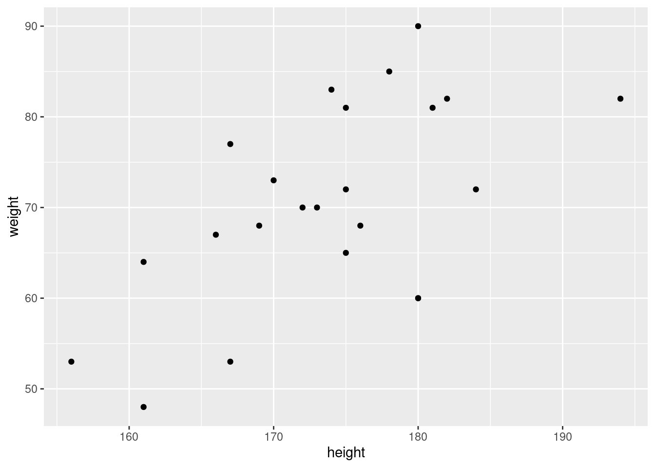

6.4 Include a regression line:

ggplot(classdata, aes(x=height, y=weight)) +
  geom_point() +
  stat_smooth(formula=y~x, method="lm", se=FALSE, colour="red", linetype=1)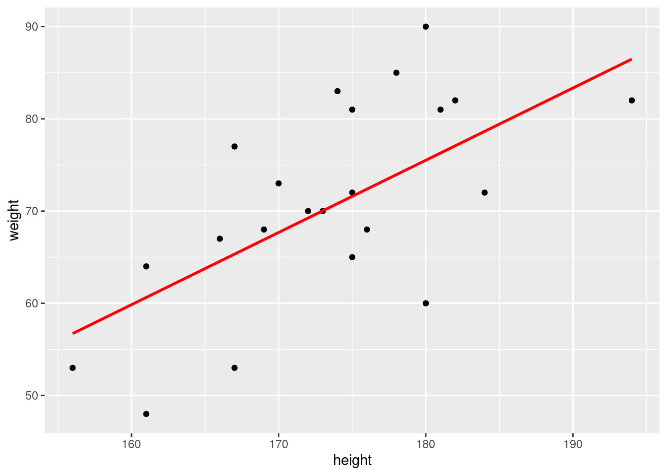

6.5 Regression: Distinguish male/female by including a seperate constant:

## baseline regression  model
model  <- lm(weight ~ height + sex , data = classdata )
show(model)


Call:
lm(formula = weight ~ height + sex, data = classdata)

Coefficients:
(Intercept)       height         sexw  
   -29.5297       0.5923      -5.7894

interm <- model$coefficients[1] 
slope  <- model$coefficients[2]
interw <- model$coefficients[1]+model$coefficients[3]

summary(model)


Call:
lm(formula = weight ~ height + sex, data = classdata)

Residuals:
    Min      1Q  Median      3Q     Max 
-17.086  -3.730   2.850   7.245  12.914 

Coefficients:
            Estimate Std. Error t value Pr(>|t|)  
(Intercept) -29.5297    47.6606  -0.620   0.5425  
height        0.5923     0.2671   2.217   0.0383 *
sexw         -5.7894     4.4773  -1.293   0.2107  
---
Signif. codes:  0 '***' 0.001 '**' 0.01 '*' 0.05 '.' 0.1 ' ' 1

Residual standard error: 8.942 on 20 degrees of freedom
Multiple R-squared:  0.4124,    Adjusted R-squared:  0.3537 
F-statistic: 7.019 on 2 and 20 DF,  p-value: 0.004904

ggplot(classdata, aes(x=height, y=weight, shape = sex)) +
  geom_point() +
  geom_abline(slope = slope, intercept = interw, linetype = 2, size=1.5)+
  geom_abline(slope = slope, intercept = interm, linetype = 2, size=1.5) +
  geom_abline(slope = coef(model)[[2]], intercept = coef(model)[[1]])

Warning: Using `size` aesthetic for lines was deprecated in ggplot2 3.4.0.
ℹ Please use `linewidth` instead.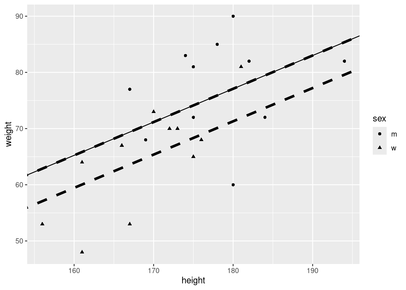

That does not look good. Maybe we should introduce also different slopes for male and female.

ggplot(classdata, aes(x=height, y=weight, shape = sex)) +
  geom_point( aes(size = 2)) +
  stat_smooth(formula = y ~ x,  method = "lm", 
              se = FALSE, colour = "red", linetype = 1)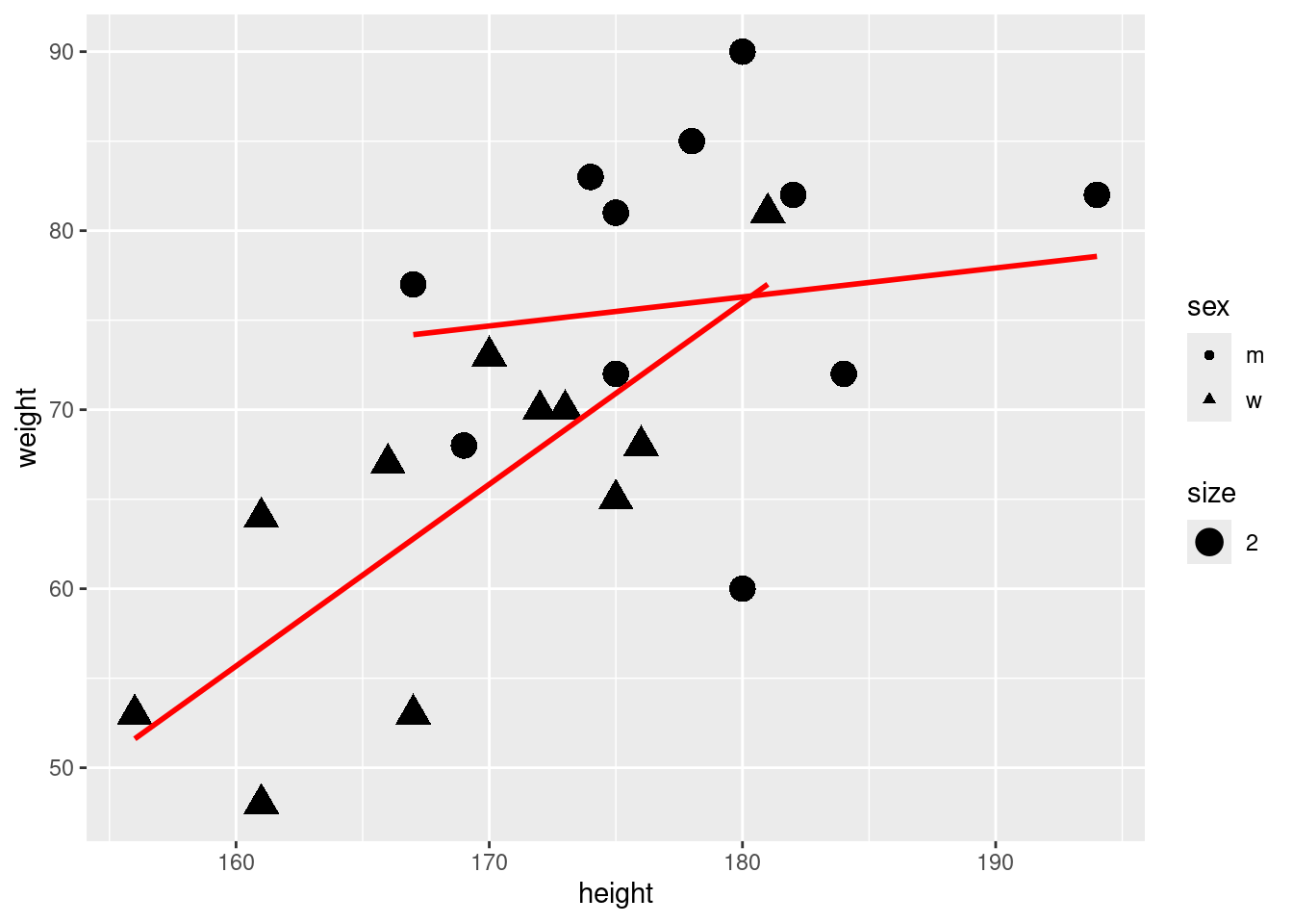

6.6 Can we use other available variables such as siblings?

ggplot(classdata, aes(x=height, y=weight, shape = sex)) +
  geom_point( aes(size = siblings))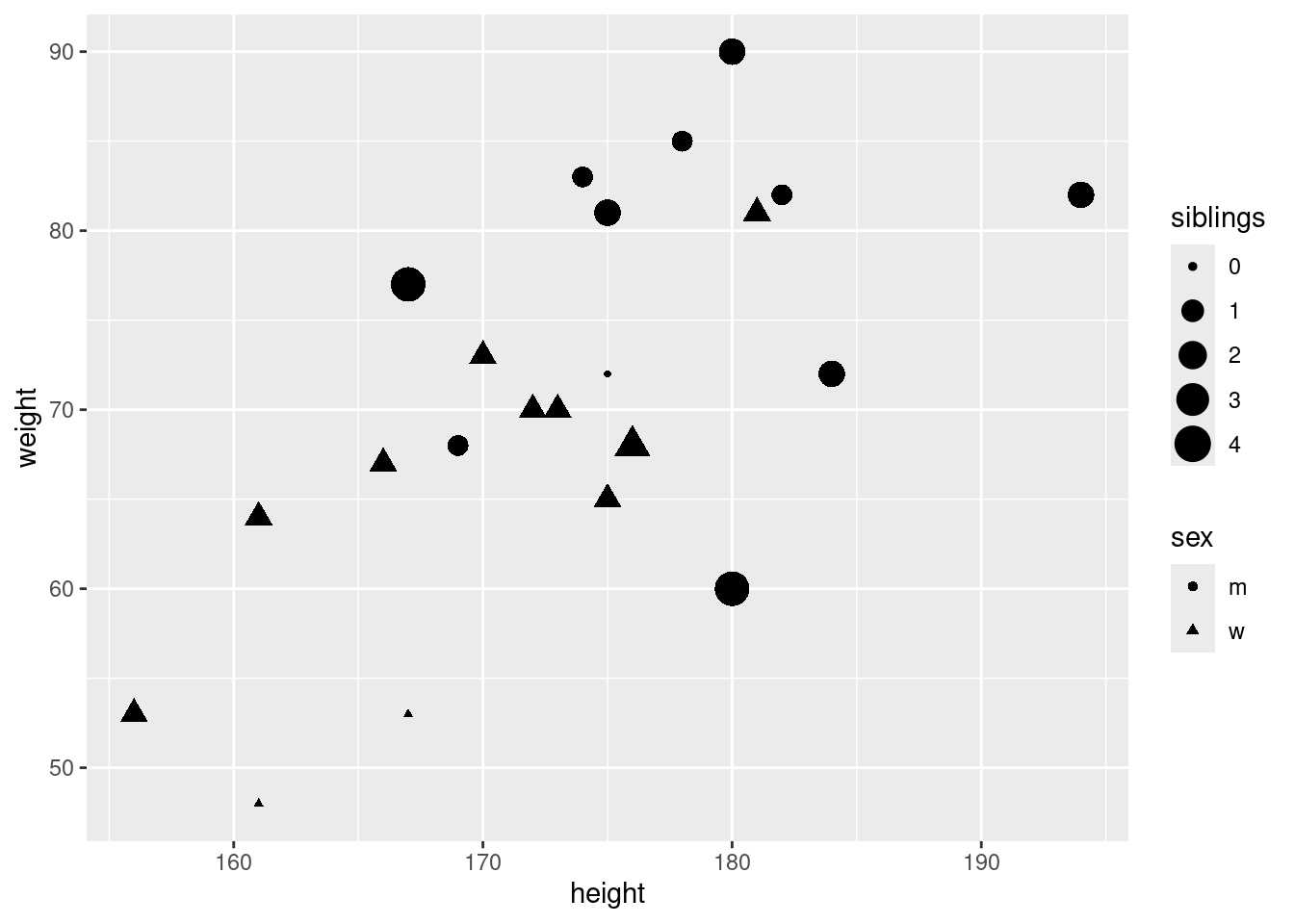

ggplot(classdata, aes(x=height, y=weight, shape = sex)) +
  geom_point( aes(size = 2)) +
  stat_smooth(formula = y ~ x,  
              method = "lm", 
              se = T, 
              colour = "red", 
              linetype = 1)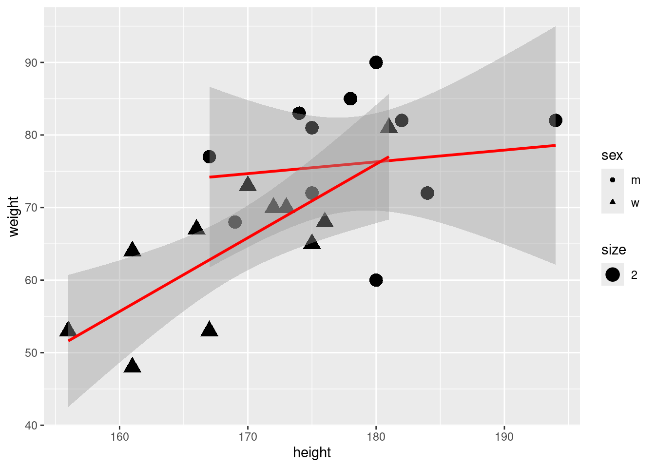

6.7 Let us look at regression output:

m1 <- lm(weight ~ height , data = classdata )
m2 <- lm(weight ~ height + sex , data = classdata )
m3 <- lm(weight ~ height + sex + height * sex , data = classdata )
m4 <- lm(weight ~ height + sex + height * sex + siblings , data = classdata )
m5 <- lm(weight ~ height + sex + height * sex , data = subset(classdata, siblings < 4 ))

6.8 Interpretation of the results

We can make predictions about the impact of height on male and female
As both, the intercept and the slope differs for male and female we should interpret the regressions seperately:
One centimeter more for MEN is on average and ceteris paribus related with 0.16 kg more weight.
One centimeter more for WOMEN is on average and ceteris paribus related with 1.01 kg more weight.

6.9 Regression diagnostics

Linear Regression makes several assumptions about the data, the model assumes that:

The relationship between the predictor (x) and the dependent variable (y) has linear relationship.
The residuals are assumed to have a constant variance.
The residual errors are assumed to be normally distributed.
Error terms are independent and have zero mean.

More on regression Diagnostics can be found Applied Statistics with R: 13 Model Diagnostics

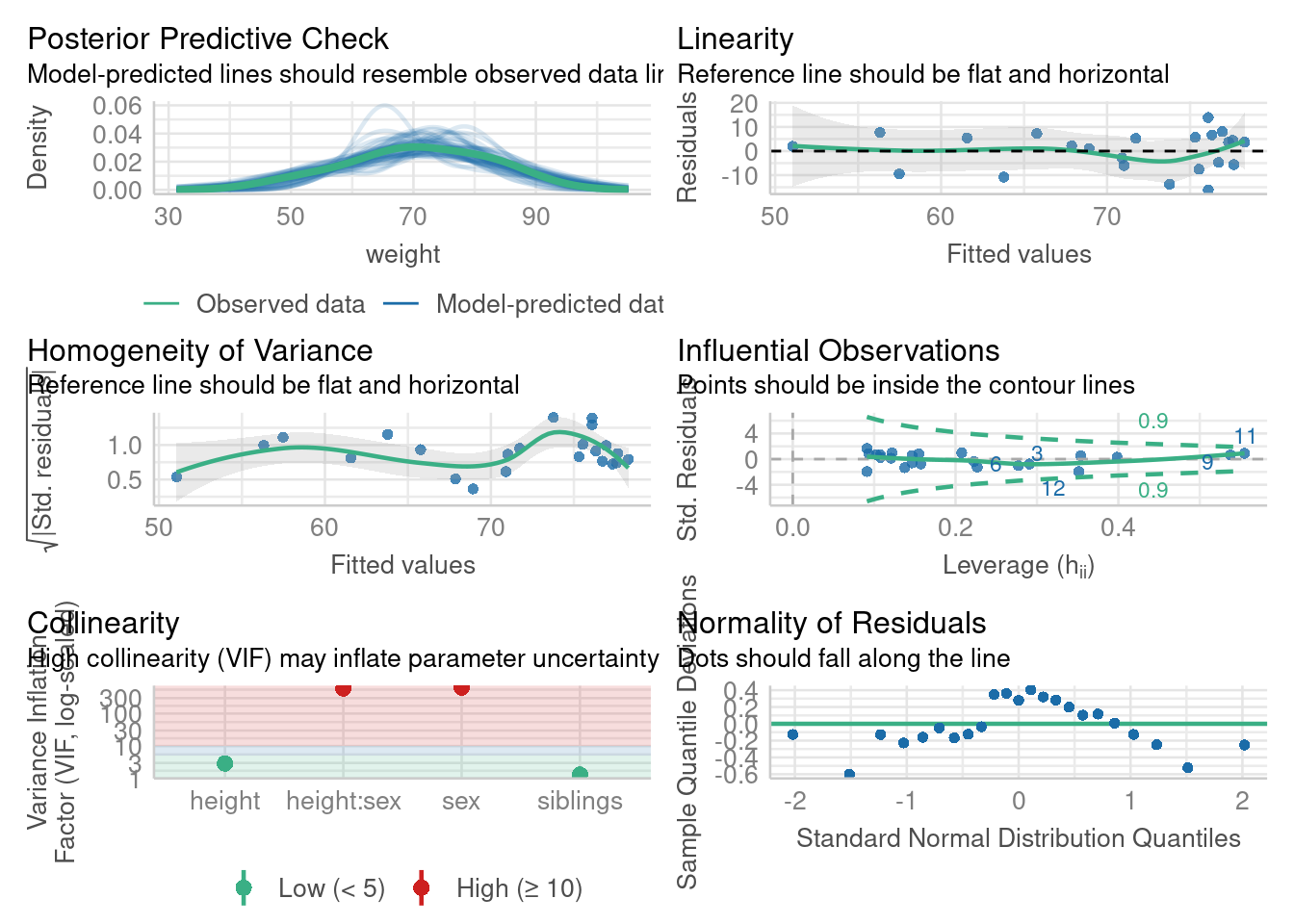
6.9.1 Check assumptions

When performing regression analysis, it is crucial to validate that the underlying assumptions of the model are met. These assumptions include linearity, independence, homoscedasticity (constant variance of residuals), absence of multicollinearity, and normality of residuals. Diagnosing these assumptions helps ensure the reliability and validity of the model.

In this section, we will explore how to perform regression diagnostics in R using the performance and see packages, which provide comprehensive tools for evaluating model assumptions and performance. Here is a sample code to illustrate these concepts:

# Load the required packages using pacman
pacman::p_load(performance, see)

# Check for heteroscedasticity (non-constant variance of residuals)
check_heteroscedasticity(m4)

OK: Error variance appears to be homoscedastic (p = 0.630).

# Check for multicollinearity (correlations among predictors)
check_collinearity(m4)

Model has interaction terms. VIFs might be inflated.
  You may check multicollinearity among predictors of a model without
  interaction terms.

# Check for Multicollinearity

Low Correlation

     Term  VIF        VIF 95% CI Increased SE Tolerance Tolerance 95% CI
   height 2.90 [  1.93,    4.90]         1.70      0.34     [0.20, 0.52]
 siblings 1.30 [  1.07,    2.37]         1.14      0.77     [0.42, 0.94]

High Correlation

       Term    VIF        VIF 95% CI Increased SE Tolerance Tolerance 95% CI
        sex 633.56 [359.01, 1118.64]        25.17  1.58e-03     [0.00, 0.00]
 height:sex 597.51 [338.60, 1054.98]        24.44  1.67e-03     [0.00, 0.00]

# Check for normality of residuals
check_normality(m4)

OK: residuals appear as normally distributed (p = 0.086).

# Check for outliers in the model
check_outliers(m4)

OK: No outliers detected.
- Based on the following method and threshold: cook (0.816).
- For variable: (Whole model)

# Evaluate overall model performance
model_performance(m4)

# Indices of model performance

AIC     |    AICc |     BIC |    R2 | R2 (adj.) |  RMSE | Sigma
---------------------------------------------------------------
171.282 | 176.532 | 178.095 | 0.496 |     0.385 | 7.719 | 8.726

# Compare performance of multiple models and rank them
compare_performance(m1, m2, m3, m4, rank = TRUE, verbose = FALSE)

# Comparison of Model Performance Indices

Name | Model |    R2 | R2 (adj.) |  RMSE | Sigma | AIC weights | AICc weights | BIC weights | Performance-Score
---------------------------------------------------------------------------------------------------------------
m3   |    lm | 0.487 |     0.407 | 7.788 | 8.568 |       0.381 |        0.240 |       0.241 |            82.70%
m4   |    lm | 0.496 |     0.385 | 7.719 | 8.726 |       0.172 |        0.046 |       0.062 |            48.51%
m2   |    lm | 0.412 |     0.354 | 8.338 | 8.942 |       0.215 |        0.260 |       0.240 |            35.23%
m1   |    lm | 0.363 |     0.333 | 8.680 | 9.084 |       0.232 |        0.454 |       0.457 |            32.72%

# Plot the performance comparison of multiple models
plot(compare_performance(m1, m2, m3, m4, rank = TRUE, verbose = FALSE))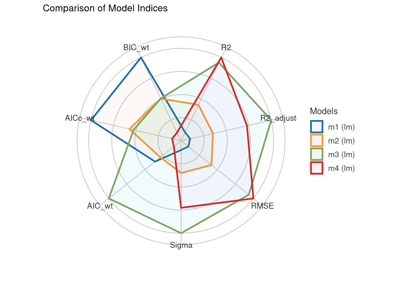

# Perform statistical tests on the model performance
test_performance(m1, m2, m3, m4)

Name | Model |    BF | df | df_diff | Chi2 |     p
--------------------------------------------------
m1   |    lm |       |  3 |         |      |      
m2   |    lm | 0.525 |  4 |    1.00 | 1.85 | 0.174
m3   |    lm |  1.00 |  5 |    1.00 | 3.14 | 0.076
m4   |    lm | 0.256 |  6 |    1.00 | 0.41 | 0.524
Models were detected as nested (in terms of fixed parameters) and are compared in sequential order.

# Comprehensive check of the model's assumptions
check_model(m4)

6.1 Making regression tables using apa_table