Appendix A — Microeconomic preliminaries
A.1 Production functions
A firm or a company is a productive unit. In particular, it is an organization that produces goods and services. In short, it can be called output. To do so, it uses inputs called factors of production, that is, labor, capital, land, skills, etc. The relationship between the inputs and the output is the production function. The goal of the firm is to achieve whatever goal its owner(s) decide to achieve through the firm. Usually, it is (and in Germany for example it has to be the case by law) to generate profits, that is, total revenue minus total cost for the level of production.
A production function (PF) is a mathematical representation of the process that transforms inputs into output.
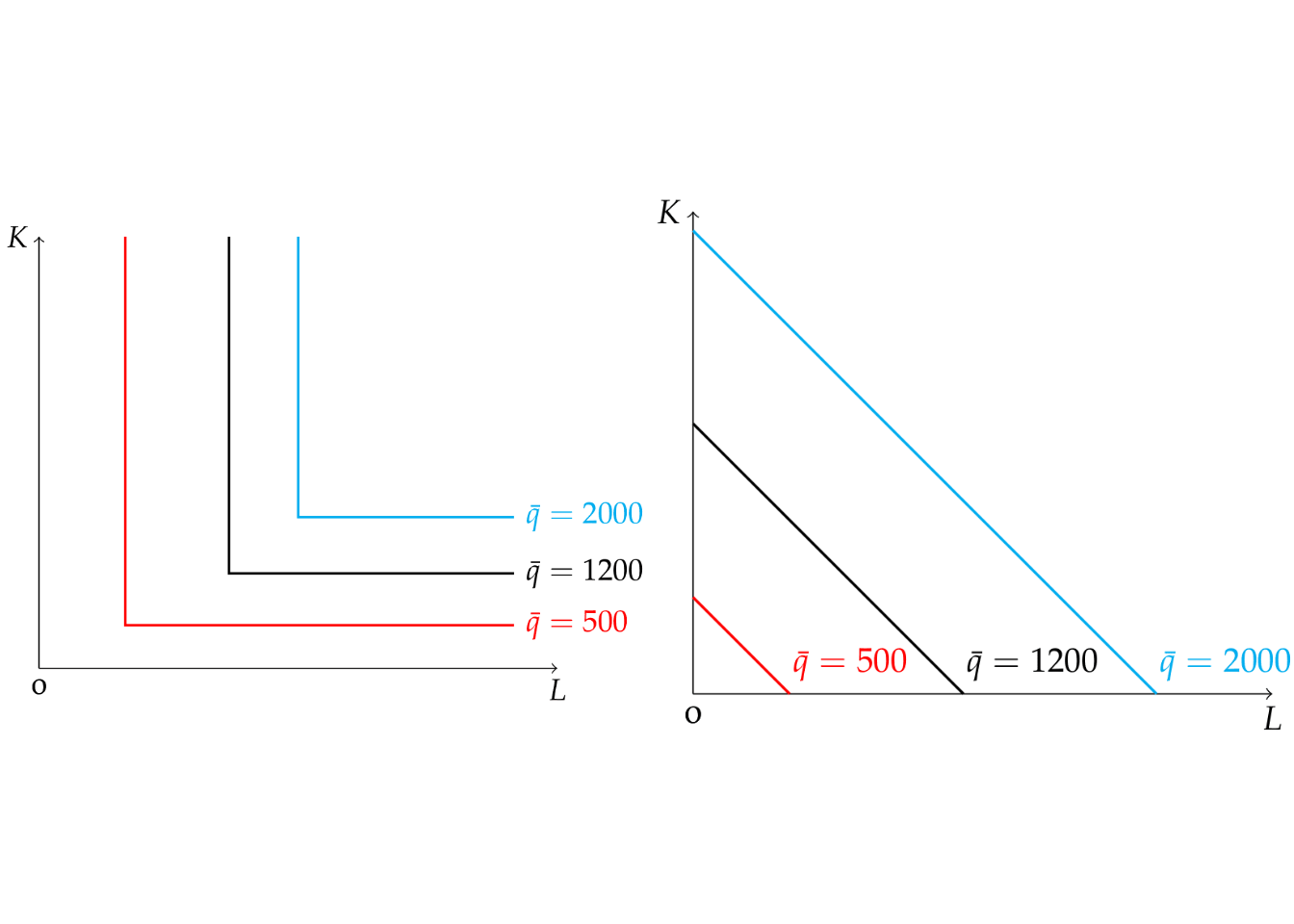
- When factors of production are perfect substitutes the PF can be written like this: \[ q=f(K,L)=L+K \]
- When factors of production are perfect complements the PF can be written like this: \[ q=f(K,L)=\min (L,K) \]
- A special and often used function is the Cobb-Douglas PF: \[ q=f(K,L)=K^\alpha L^{1-\alpha} \quad \text{with} \quad 0<\alpha<1 \]
The returns to scale describes the increase in output when a firm multiples all of its inputs by some factor. Let \(\lambda>1,\) then, with two factors \(\mathrm{K}\) and \(L\), we can define that for \[ f(c K, c L)= c^\lambda f(K, L), \]
- \(\lambda>1\) the PF has increasing returns to scale,
- \(\lambda=1\) the PF has constant returns to scale,
- \(\lambda<1\) the PF has decreasing returns to scale.
The marginal product is the change in the total output when the input varies of one infinitesimal small unit. Graphically, the marginal product is the slope of the total product function at any point. The slope of the total product function, that is, the marginal product, is generally not constant. The marginal product to an input is assumed to decrease beyond some level of input. This is called the law of diminishing marginal returns. In particular, we can distinguish:
- positive marginal returns when \(f'>0\) and
- diminishing marginal returns when \(f''<0\) and
- increasing marginal returns when \(f''>0\).
A.2 Production possibility frontier curve
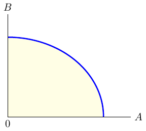
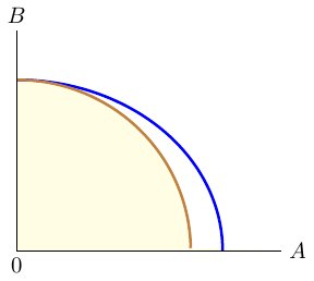
The production possibilities frontier (PPF) curve shown in Figure A.1 provides a graphical representation of all possible production options for two products when all available resources and factors of production are fully and efficiently utilized within a given time period. The PPF serves as a boundary between combinations of goods and services that can be produced and those that cannot.
The PPF is an invaluable tool for illustrating the effects of scarcity as it provides insights into production efficiency, opportunity costs and the trade-offs between different choices. In general, the PPF exhibits concavity, as not all factors of production can be used equally productively in all activities.
Economic growth refers to the continuous expansion of production possibilities. An economy experiences growth through technological advances, improvements in the quality of labor or an increase in the factors of production (labor, capital). When the resources of an economy increase, the production possibilities also expand, shifting the PPF outwards. It is worth noting that PPF can be used to explain production in an economy or company.
Production efficiency occurs when it is impossible to produce more of one good or service without producing less of another. If production takes place directly on the PPF, this means efficiency. If, on the other hand, production takes place within the PPF (yellow shaded area of Figure A.1), it is possible to produce more goods without sacrificing existing goods, which indicates inefficiency. If production is on the PPF, there is a trade-off, as obtaining more of one good requires sacrificing a certain amount of another good. This trade-off is associated with costs called opportunity costs.
Exercise A.1 Understanding production (Solution A.1)
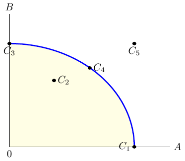
- Figure A.2 shows a PPF and five conceivable production points, \(C_i\), where \(i\in \{1,\dots,5\}\). Explain the figure using the following terms: _attainable point; available resources, unattainable, inefficient, efficient point.
What would happen to the PPF if the technology available in a country and needed for the production process became better?
What would happen to the PPF if the resources available in a country and needed in the production process of both goods shrank?
What would happen to the PPF if the resources (technology) available in a country that are needed in the production process…
- …for both goods increased (improved)?
- …for good A shrank (got worse)?
- …for good B increased (improved)?
Does the shape of the PPF tell us anything about economies of scale in the production process?
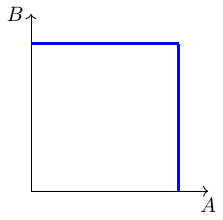
Figure A.3 shows an extreme PPF. How can such a PPF be explained?
Solution A.1. Understanding production (Exercise A.1)
Any point that lies either on the production possibilities curve or to the left of it is said to be an attainable point: it can be produced with currently available resources. Production points that lie in the yellow shaded area are said to be unattainable because they cannot be produced using currently available resources. These points represent an inefficient production, because existing resources would allow for production of more of at least one good without sacrificing the production of any other good. An efficient point is one that lies on the production possibilities curve. At any such point, more of one good can be produced only by producing less of the other.
The PPF would shift outwards.
The PPF would shift inwards.
The PPF would shift…
- …outwards for both goods.
- …inwards for good A, see Figure A.4.
- …outwards for good B.
With economies of scale, the PPF would curve inward, with the opportunity cost of one good falling as more of it is produced. A straight-line (linear) PPF reflects a situation where resources are not specialized and can be substituted for each other with no added cost. With constant returns to scale, there are two opportunities for a linear PPF: if there was only one factor of production to consider or if the factor intensity ratios in the two sectors were constant at all points on the production-possibilities curve.
Here is one example: Suppose a country that is endowed with two factors of production and that one factor can only be used for producing good A and the other factor can only be used to produce good B.
A.3 Indifference curves and isoquants
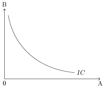
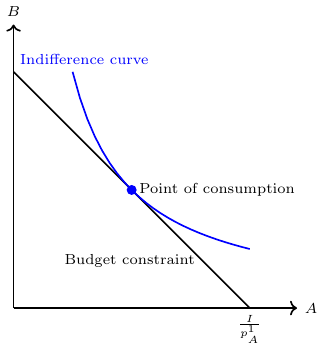
Combinations of two goods that yield the same level of utility for consumers are represented by indifference curves, see figure Figure A.5. These curves illustrate the various bundles of goods where consumers are equally satisfied. That means all points on an indifference curve represent the same level of utility. The shape of the indifference curve is determined by the underlying utility function, which captures the preferences of consumers for consuming different combinations of the two goods.
The slope of an indifference curve indicates the rate at which the two goods can be substituted while maintaining the same level of utility for the consumer. Technically, the slope represents the marginal rate of substitution, which is equal to the absolute value of the slope. It measures the maximum quantity of one good that a consumer is willing to give up in order to obtain an additional unit of the other good.
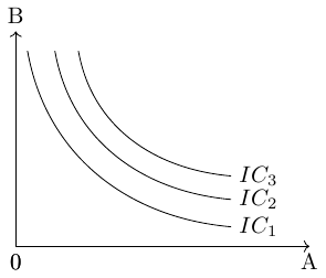
It is assumed that consumers aim to attain the highest possible indifference curve because a higher curve, located further to the right on a coordinate system, represents a higher level of utility. In Figure A.6, for example, \((IC_1)\) represents a lower level of utility than \((IC_2)\).
Similar to the concept of indifference curves, an isoquant shows the combinations of factors of production that result in the same quantity of output.
A.4 Budget constraint
In microeconomics, the concept of a budget constraint plays a vital role in understanding consumer decision-making and helps to analyze consumer choices and trade-offs. The budget constraint represents the limitations faced by consumers in allocating their limited income across different goods and services. The budget constraint indicates that the total expenditure on goods and services, calculated by multiplying the prices of each item by its corresponding quantity, must be less than or equal to the consumer’s income. Mathematically, the budget constraint can be expressed as: \[ P_1 \cdot Q_1 + P_2 \cdot Q_2 + \ldots + P_n \cdot Q_n \leq I \] where (\(P_n\)) represent the prices of goods, (\(Q_n\)) denote the quantities of goods (\(n\)) consumed. (\(I\)) denotes the consumer’s income or their budget.
Consumers strive to maximize their utility by selecting the optimal combination of goods and services within the constraints imposed by their limited income. This involves making decisions about how much of each good to consume while staying within the budgetary limits. The graphical representation of the ideal consumption point is depicted in Figure Figure A.8.
By studying the budget constraint, economists can gain insights into consumer behavior, price changes, and the impact of income fluctuations on consumption patterns.