2 International trade
Trade is usually a voluntary decision by buyers and sellers, which means that transactions would not take place if one party were to lose from the exchange. While this reasoning is persuasive, it alone does not fully justify unrestricted international trade. In the following chapters, we will look at the concept that trade should be mutually beneficial to the parties directly involved. We will also discuss the ways in which trade can be beneficial to all parties, even though it is not necessarily beneficial to all. The remainder is structured as follows:
- Section 2.1 explains Mankiw’s principle that trade can make everyone better off.
- Section 2.2 paraphrases the sources of international trade.
- Section 2.3 provides a theoretical framework of trade and shows that under certain circumstances international trade can yield a miserable growth path for a country.
- Section 2.4 explains that more trade does not have to be good for a country’s wealth.
- Section 2.5 introduces the concept of comparative advantage. It claims that trade is due to autarky price differences that stem from country-specific differences such as technology, factor endowments, or taste.
- Section 2.6 shows that opening up to free trade generates winners and losers and that countries’ endowments with labor and capital determine patterns of trade.
2.1 Trade can make everyone better off

Source: Harvard.edu and Mankiw (2024).
N. Gregory Mankiw (*1958) is one of the most influential economists. In his best-selling textbook Principles of Economics (Mankiw, 2024, pp. 8–9) he claims ten principles of economics of which one is entitled Trade can make everyone better off which he explains as follows:
You have probably heard on the news that the Japanese are our competitors in the world economy. In some ways, this is true, for American and Japanese firms do produce many of the same goods. Ford and Toyota compete for the same customers in the market for automobiles. Compaq and Toshiba compete for the same customers in the market for personal computers.
Yet it is easy to be misled when thinking about competition among countries. Trade between the United States and Japan is not like a sports contest, where one side wins and the other side loses. In fact, the opposite is true: Trade between two countries can make each country better off.
To see why, consider how trade affects your family. When a member of your family looks for a job, he or she competes against members of other families who are looking for jobs. Families also compete against one another when they go shopping, because each family wants to buy the best goods at the lowest prices. So, in a sense, each family in the economy is competing with all other families.
Despite this competition, your family would not be better off isolating itself from all other families. If it did, your family would need to grow its own food, make its own clothes, and build its own home. Clearly, your family gains much from its ability to trade with others. Trade allows each person to specialize in the activities he or she does best, whether it is farming, sewing, or home building. By trading with others, people can buy a greater variety of goods and services at lower cost.
Countries as well as families benefit from the ability to trade with one another. Trade allows countries to specialize in what they do best and to enjoy a greater variety of goods and services. The Japanese, as well as the French and the Egyptians and the Brazilians, are as much our partners in the world economy as they are our competitors.
2.2 Reasons for Trade
Trade involves willingly giving up something to receive something else in return, which should benefit both parties involved, although not necessarily everyone affected by the trade. We will discuss the negative effects of international trade on bystanders later. In this section, we briefly outline basic reasons for individuals and hence countries to engage in trade. Of course, the list is incomplete.
Differences in Technology: Advantageous trade can occur between countries if they have different technological abilities to produce goods and services. Technology refers to the techniques used to convert resources (labor, capital, land) into outputs. Differences in technology form the basis for trade in the Ricardian Model of comparative advantage. We will revisit this in more detail in Section 2.5.
Differences in Endowments: Trade also occurs because countries differ in their resource endowments, which include the skills and abilities of the workforce, available natural resources, and the sophistication of capital stock such as machinery, infrastructure, and communication systems. Differences in resource endowments are the basis for trade in the pure exchange models (see Section 2.3) and the Heckscher-Ohlin Model (see Section 2.6).
Differences in Demand: Trade between countries occurs because demands or preferences differ. Individuals in different countries may prefer different products even if prices are the same. For example, Asian populations might demand more rice, Czech and German people more beer, the Dutch more wooden shoes, and the Japanese more fish compared to Americans.
Economies of Scale in Production: Economies of scale, where production costs fall as production volume increases, can make trade between two countries advantageous. This concept, known as increasing returns to scale, plays a significant role in Paul Krugman’s New Trade Theory, which we will discuss later.
Existence of Government Policies: Government tax and subsidy programs can create production advantages for certain products, leading to advantageous trade arising solely from differences in government policies across countries. We will explore the impact of tariffs and regulations in Chapter 3.
2.3 Exchange economy
2.3.1 A simple barter model
The simplest example to show that trade can be beneficial to people is the barter model. In trade, barter is a system of exchange in which participants in a transaction directly exchange goods or services for other goods or services without using a medium of exchange, such as money.

Source: Wikipedia
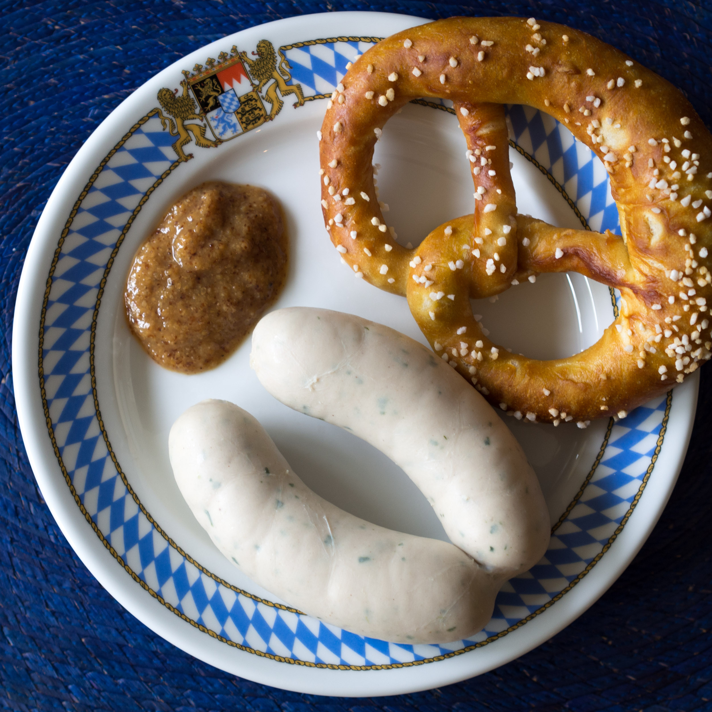
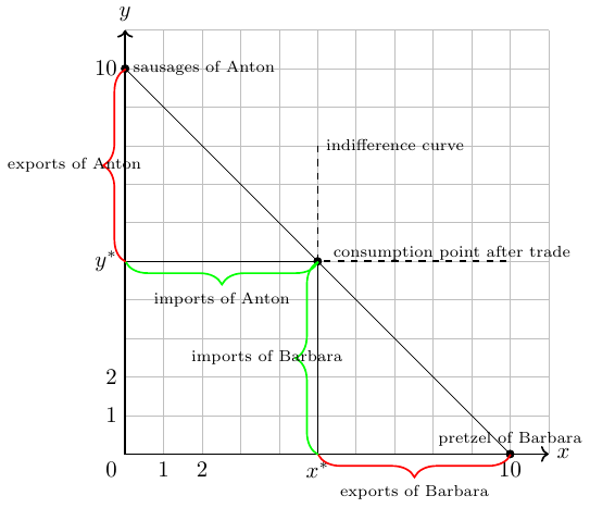
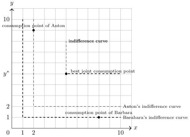
Suppose there are two people, Anton (A) and Barbara (B). Anton has 10 Weißwürste (white sausages) and Barbara has 10 pretzels. Together, they are isolated from the rest of the world for a few days due to a natural disaster. Fortunately, they both have additional access to an endless supply of sweet mustard and beer and they now wonder how to share pretzels and sausages the upcoming days. Let’s assume that both of them accept only a white sausage eaten together with a pretzel. That is, eating two pretzels with a sausage is no better than eating a pretzel and a sausage. After some discussion, Barbara gives 5 pretzels and Anton gives Barbara 5 sausages in return. They strongly believe that there is no better way to share food.
This example shows that trade can be beneficial for two individuals. Here we basically assume two things. Firstly, two individuals can trade and secondly, they are endowed with different goods.
Solution 2.1. How Barbara and Anton trade (Exercise 2.1)
In Figure 2.3 you find a sketch of a solution to tasks a. to c. Figure 2.4 provides a solution to task d.
2.3.2 Terms of trade
The terms of trade is defined as the quantity of one good that exchanges for a quantity of another. It is typical to express the terms of trade as a ratio.
In the example of Barbara and Anton, the exchange of goods occurs at a 1:1 ratio. In economics, this is referred to as the terms of trade being 1. The terms of trade are defined as the relative price of exports in relation to imports, or in other words, how much of one good can be exchanged for another. For instance, determining how many sausages can be exchanged for how many pretzels. The terms of trade, determined by the two trading partners, depend on a variety of distinct factors, including:
Preferences: For trade to occur, each trader must desire something the other has and be willing to give up something of their own to obtain it. Formally, the expected utility of consuming some of Anton’s bread must exceed the disutility of foregoing a few of his sausages, and vice versa for Barbara. Typically, the goods are substitutable rather than perfectly complementary, as is assumed in our specific example.
Uncertainty: Both individuals have clear preferences. If Barbara has never tried Anton’s sausages, and Anton typically prefers bread over pretzels, offering free samples before an exchange could reduce uncertainty. Without a sample, their trade would be based on expectations about the taste of the other’s product.
Scarcity: The availability of the two goods influences the terms of trade. If, for instance, Barbara has 1000 pretzels, the terms of trade with the sausages would likely change.
Size: The physical size of the goods can impact the terms of trade.
Quality: The quality of goods affects the terms of trade. If the pretzels are stale and hard, both might prefer fewer pretzels per sausage.
Persuasion: If Barbara is a more persuasive salesperson than Anton, she might be able to negotiate more favorable terms of trade.
Government Policy: Taxes imposed by an official based on the traded quantities could affect the terms of trade. Additionally, if laws prevent Barbara and Anton from meeting, no trade would occur.
Exercise 2.2 Terms of trade (?sol-Termsoftrade)
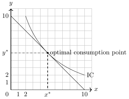
Suppose you have a fixed income \(I=10\) that you can spend on consuming two substitutable goods \(x, y\) at certain prices \(p_x=1, p_y=1\). The current consumption decission is sketched in the figure above. Suppose the price of good \(x\) increases, that is, \(p_x=2\). Draw the new budget line. How will consumption change? What are the new terms of trade?
The new point of optimal consumption \(OCP_1\) at \((x=2,y=6)\) illustrates that an increase in the price of good \(x\) leads consumers to substitute good \(x\) and consume more of good \(y\) but less of good \(x\).
The terms of trade are now \(\frac{p_x}{p_y}=2\). That is, consumers are willing to give up 1 unit of good \(x\) to receive 2 units of good \(y\). The budget line is drawn in blue.
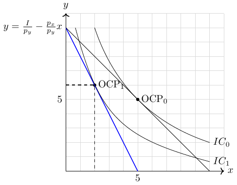
Note: The indifference curve \(IC_1\) in the graph is just a guess of mine because we don’t have preferences in form of a utility function given. For example, you can also draw an indifference curve that gives you the optimal consumption point at \((x= 1;y= 8)\) or \((x= 4;y= 2)\).
2.3.3 Endowments in an Exchange Economy
In this section, we examine a basic scenario where productive units within an economy are unable to adjust their output to recent changes in world market prices, which stem from global demand and supply fluctuations. Economists refer to the resulting availability of goods as endowments. Essentially, a country is endowed with a certain quantity of goods and seeks to trade these goods on global markets to maximize its welfare. In Section 2.6 we will assume that countries are endowed with a certain amount of factors of production that they can use to produce various goods.
2.3.3.1 Fixed production
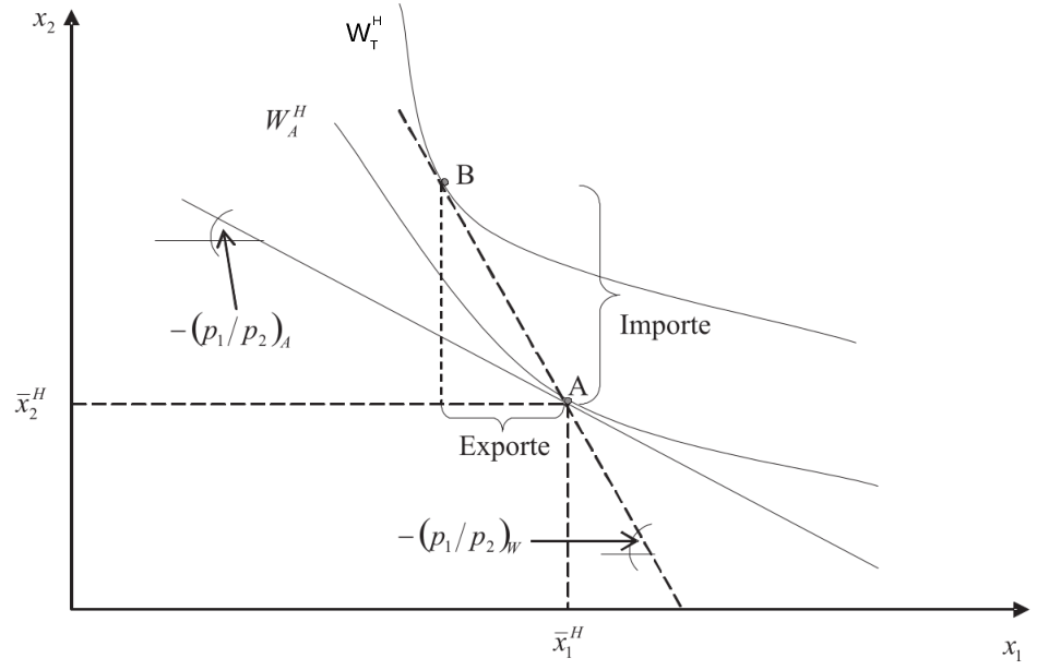
Imagine that country H produces \(\bar{x}^H_1\) units of good 1 and \(\bar{x}^H_2\) units of good 2. In autarky (a state of where there is no trade), it consumes all the goods it produces. This scenario is shown in Figure 2.7, where point A represents the optimal welfare outcome with utility \(W^H_A\) for country H in autarky.
Now, let’s assume country H can trade with the rest of the world at global market prices, where the price ratio of good 1 to good 2 in the world market, \(( \frac{p_1}{p_2} )_W\), is greater than in autarky, \(( \frac{p_1}{p_2} )_A\): \[\begin{align} \left( \frac{p_1}{p_2} \right)_W > \left( \frac{p_1}{p_2}\right)_A, \end{align}\]
With trade, country H can achieve a higher utility, \(W_T^H>W_A^H\), by exporting good \(x_1\) and importing good \(x_2\), thus moving to a more advantageous consumption point.
2.3.3.2 Flexible production
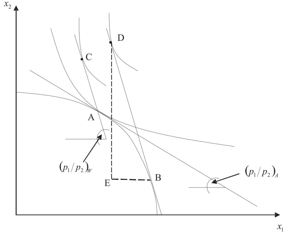
- Trade is even more beneficial to a country if it can adjust its production to export more goods that are relatively high priced in the world market. This statement is shown in Figure 2.8.
- In autarky, optimal consumption would be at point A and optimal consumption would be at point C under free trade. Now suppose that producers in country H know that they can sell their goods at price \(p_1^W\) and \(p_2^W\) before deciding what to produce. Then they would choose production point B on the production frontier curve to export good \(x_1\) and import good \(x_2\) at price \((\frac{p_1}{p_2})_A\) to be consumed at point D. Welfare at point D is higher than at point C or A because we end up at the highest indifference curve.
Exercise 2.3 Production and consumption
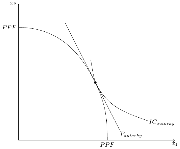
In Figure 2.9 the production possibility frontier curve, \(PPF\), of a country, \(H\), in autarky in which only two products, \(x_1\) and \(x_2\), can be produced and consumed, respectively.
Given the country is in autarky (that is, no trade), the price relation of both goods within the country is represented by the line denoted with \(P_{autarky}\). The indifference curve that represents the utility maximizing level of utility is denoted with \(IC_{autarky}\). Mark in the figure how much of both goods are produced and consumed, respectively.
Suppose country \(H\) opens up to trade with foreign countries. Further assume that the country can trade with other countries at fixed world market prices
\[\begin{align} \left(\frac{p_1}{p_2}\right)_W>\left(\frac{p_1}{p_2}\right)_A, \end{align}\] where \((\frac{p_1}{p_2})_A\) denotes the price relation of country H in autarky, \(P_{autarky}\). Sketch the world market price relation in the figure and mark the new production point on the production possibility frontier curve. Moreover, mark below those statements that are true:Country \(H\) will produce more of good \(x_1\) than in autarky
Country \(H\) will produce more of good \(x_2\) than in autarky
Country \(H\) will consume more of good \(x_1\) than in autarky
Country \(H\) will export good \(x_1\) and import good \(x_2\).
Country \(H\) will export good \(x_2\) and import good \(x_1\).
Country \(H\) will suffer a loss of welfare due to opening up to trade.
Exercise 2.4 Production and consumption (?sol-gains)
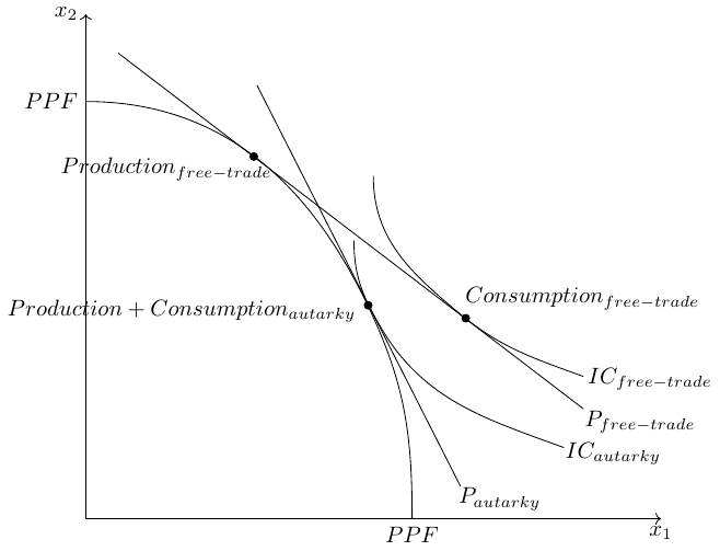
Show that opening markets to foreign trade can be beneficial for a small economy where only two goods can be produced and consumed. Use a two-way diagram to do this. In particular, show the consumption and production point of the economy in autarky with the corresponding price relation. Then assume that the economy opens up to the foreign market, allowing it to buy goods at world prices that are different from prices in autarky. Show the consumption and production point of the autarkic economy with the corresponding price relation under free trade. Can you outline the higher level of welfare in free trade?
As visualized in Figure 2.10, the indifference curve under free trade lies above the IC under autarky. This reflects the higher utility level under free trade.
2.4 More trade is not necessarily good (immiserizing growth)
So far, I have implicitly assumed that the world market price is fixed and not changed by the entry of country H into the free trade market. When the latter is the case, economists speak of a small open economy (SOE). In general, a SOE is an economy that is so small that its policies do not change world prices.
Suppose that country H is not an SOE. What would happen to world prices if country H offered a lot of good \(x_1\) to receive good \(x_2\)? Obviously, \((\frac{p_1}{p_2})_W\) would fall. In the worst case, country H is so large that \[\left(\frac{p_1}{p_2}\right)_W=\left(\frac{p_1}{p_2}\right)_A.\] This means that country H has no benefits from free trade.
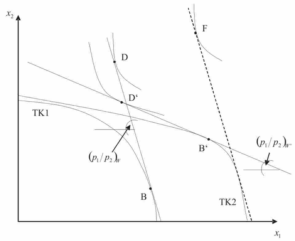
Assuming that a (large) country cannot opt out from free trade and that the exporting sector grows, there is a theoretical scenario called immiserizing growth that shows that free trade countries are worse off in the long run. This scenario is illustrated in Figure 2.11. The figure summarizes two periods. In the first period, country H produces at point B and consumes at point D, trading goods at world prices \((\frac{p_1}{p_2})_W\). Then country H grows in sector 1. This is shown in the new production possibility curve TK2. If country H were able to trade at the old world price, it would be able to consume at point F. Unfortunately, country H is not a SOE, and therefore world prices (from country H’s perspective) deteriorate to \((\frac{p_1}{p_2})_W^{'}\). This has bad implications for country H, since its optimal consumption is now at point D’, which has lower welfare relative to point D. However, this is not an argument against trade, since the welfare at point D’ is still above the production possibility curve in autarky, TK1.
2.5 The theory of comparative advantage (Ricardian Model)
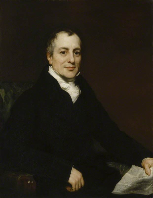
Source: National Portrait Gallery
David Ricardo (1772-1823), one of the most influential economists of his time, had a simple idea that had a major impact on how we think about trade. In Ricardo (1817), he argued that bilateral trade can be a positive-sum game for both countries, even if one country is less productive in all sectors, if each country specializes in what it can produce relatively best.
1 Actually, strictly speaking, this is not correct, since the original description of the idea can already be found in Torrens (1815). However, David Ricardo formalized the idea in his 1817 book using a convincing and simple numerical example. For more information on this, as well as a great introduction to the Ricardian model and more, I recommend Suranovic (2012).
He introduced the theory of comparative advantage that is still an important corner stone of the modern theory of international trade1 It refers to the ability of one party (an individual, a firm, or a country) to produce a particular good or service at a lower opportunity cost than another party. In other words, it is the ability to produce a product with the highest relative efficiency, given all other products that could be produced. In contrast, an absolute advantage is defined as the ability of one party to produce a particular good at a lower absolute cost than another party.

As shown in Figure 2.13, the concept of comparative advantage is quite simple. Two parties can increase their overall productivity by sharing the workload based on their respective comparative advantages. Once they have achieved this increase in productivity, they must agree on how to divide the resulting output. Of course, both parties must benefit compared to a scenario in which they work independently.
2.5.1 Defining absolute and comparative advantages
A subject (country, household, individual, company) has an absolute advantage in the production of a good relative to another subject if it can produce the good at lower total costs or with higher productivity. Thus, absolute advantage compares productivity across subjects but within an item.
A subject has a comparative advantage in the production of a good relative to another subject if it can produce that good at a lower opportunity cost relative to another subject.
Let me explain the idea of the concept of comparative advantage with some examples:
Old and young
Two women live alone on a deserted island. In order to survive, they have to do some basic activities like fetching water, fishing and cooking. The first woman is young, strong and educated. The second is older, less agile and rather uneducated. Thus, the first woman is faster, better and more productive in all productive activities. So she has an absolute advantage in all areas. The second woman, in turn, has an absolute disadvantage in all areas. In some activities, the difference between the two is large; in others, it is small. The law of comparative advantage states that it is not in the interest of either of them to work in isolation: They can both benefit from specialization and exchange. If the two women divide the work, the younger woman should specialize in tasks where she is most productive (for example, fishing), while the older woman should focus on tasks where her productivity is only slightly lower (for example, cooking). Such an arrangement will increase overall production and benefit both.
The lawyer’s typist
The famous economist and Nobel laureate Paul Samuelson (1915-2009) provided another example in his well-received textbook of economics, as follows: Suppose that in a given city the best lawyer also happens to be the best secretary. However, if the lawyer focuses on the task of being a lawyer, and instead of practicing both professions at the same time, hires a secretary, both the lawyer’s and the secretary’s performance would increase because it is more difficult to be a lawyer than a secretary.2
2 In the first eight editions the example comprised a male lawyer who was better at typing than his female secretary, but who had a comparative advantage in practising law. In the ninth edition published 1973, both lawyer and secretary were assumed to be female (see Backhouse & Cherrier, 2019). Unfortunately, women are still discriminated against in introductory economics textbooks (see Stevenson & Zlotnik, 2018).
2.5.2 Autarky: An example of two different persons
Assume that A and B want to produce and consume \(y\) and \(x\) respectively. Because of the complementarity of the two goods, each must be consumed in combination with the other. The utility function of both persons is \(U_{\{A;B\}}=min(x,y)\). Both persons work for 4 time units, that is, their units of labor are \(L_A=L_B=4\). A needs 1 units of labor to produce one unit of good \(y\) and 2 units of labor to produce one unit of good \(x\). B needs \(\frac{4}{10}=0.4\) units of labor to produce one unit of good \(y\) or good \(x\). Thus, their labor input coefficients, which measure the units of labor required by a subject to produce one unit of good, are \(a^A_y=1, a^A_x=2, a^B_y=0.4, a^B_x=0.4\):
| input coefficient (\(a\)) | A | B |
|---|---|---|
| Good \(y\) | 1 | 0.4 |
| Good \(x\) | 2 | 0.4 |
Spending all her time in the production of \(y\), A can produce \(\frac{L_A}{a_y^A}=\frac{4}{1}=4\) units of \(y\) and B can produce \(\frac{L_B}{a_y^B}=\frac{4}{0.4}=10\) units of \(y\). Spending all her time in the production of \(y\), A can produce \(\frac{L_A}{a_x^A}=\frac{4}{2}=2\) units of \(x\)and B can produce \(\frac{L_B}{a_x^B}=\frac{4}{0.4}=10\) units of \(x\). Knowing this, we can easily draw the production possibility frontier curves (PPF) of person A and B as shown in Figure 2.14.
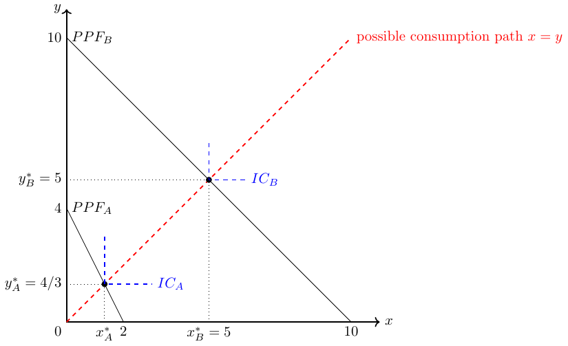
In autarky, both person maximize their utility: Individual A can consume \(\frac{4}{3}\) units of each good and individual B can consume \(5\) units of each good. The respective indifference curves are drawn in dashed blue lines in Figure 2.14.
2.5.2.1 Can person A and B improve their maximum consumption with cooperation?
Let us assume the two persons come together and try to understand how they can improve by jointly deciding which goods they should produce. If we assume that both persons redistribute their joint production so that both have an incentive to share and trade, we can concentrate on the total production output. Their joint PPF curve can then be drawn in two ways:
- Person A specializes in good \(x\), then the joint production possibilities are presented in Figure 2.15.
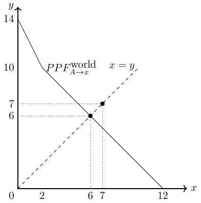
If A produces only good \(x\), as shown in Figure 2.15, we see that A and B can consume a total of 6 units of goods \(x\) and \(y\). This is less in total than in autarky, where A can consume \(\frac{4}{3}\) units of each good and person B can consume \(5\) units of each good, giving a combined consumption of \(\frac{19}{3}=6,\bar{6}\).
- Person A specializes in good \(y\), then the joint production possibilities are presented in Figure 2.16.
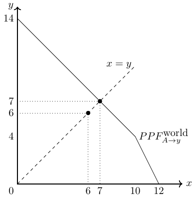
If A produces only good \(y\), as shown in Figure 2.16, we see that A and B can consume a total of 7 units of goods \(x\) and \(y\). Thus, both can be better off compared to autarky, since the total quantity distributed is larger. Thus, we have an Pareto improvement here because at least one person can be better off compared to autarky.
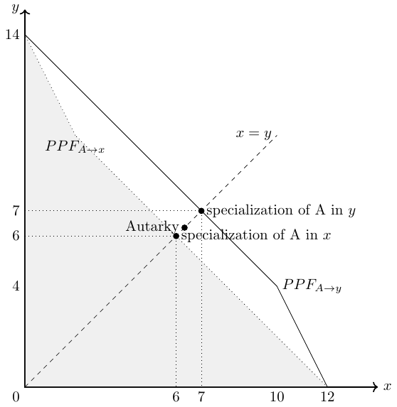
In Figure 2.17, the three possible consumption scenarios are marked with a dot and the PPFs of person A specializing in the production of good \(x\) (\(PPF_{A\rightarrow x}\)) or good \(y\) (\(PPF_{A\rightarrow y}\)) are also drawn. The scenario with person A specializing in the production of good \(y\) is the output maximizing solution.
2.5.2.2 Optimal production in cooperation
In order to produce the most bundles of both goods, the optimal cooperative production is
| production in cooperation | A | B |
|---|---|---|
| Good \(y\) | 4 | 3 |
| Good \(x\) | 0 | 7 |
2.5.2.3 Check for absolute advantage
Employing 10 units of labor B can produce more of both goods and hence has an absolute advantage in producing \(x\) and \(y\). Formally, we can proof this by comparing the input coefficients of both countries in each good:
| absolute advantage | A | B | ||
|---|---|---|---|---|
| Good \(y\) | \(a_y^A=1\) | > | \(0.4=a_y^B\) | \(\Rightarrow\) B has an absolute advantage in good \(y\) |
| Good \(x\) | \(a_x^A=2\) | > | \(0.4=a_x^B\) | \(\Rightarrow\) B has an absolute advantage in good \(x\) |
2.5.2.4 Check for comparative advantage
The slope of the PPFs represent the marginal rate of transformation, the terms of trade in autarky and the opportunity costs of a country. The opportunity costs are defined by how much of a good \(x\) (or \(y\)) a person (or country) has to give up to get one more of good \(y\) (or \(x\)). For example, A must give up \(\frac{a_x^A}{a_y^A}=\frac{1}{2}=0.5\) of good \(x\) to produce one more of good \(y\). Thus, A’s opportunity costs of producing one unit of \(y\) is the production foregone, that is, a half good \(x\). All opportunity costs of our example are:
| opportunity costs of producing … | A | B |
|---|---|---|
| …1 unit of good \(y\): | \(\frac{a_y^A}{a_x^A}=\frac{1}{2}=0.5\) (good x) | \(\frac{a_y^B}{a_x^B}=\frac{0.4}{0.4}=1\) (good x) |
| …1 unit of good \(x\): | \(\frac{a_x^A}{a_y^A}=\frac{2}{1}=2\) (good y) | \(\frac{a_x^B}{a_y^B}=\frac{0.4}{0.4}=1\) (good y) |
Person A has a comparative advantage in producing good \(y\) since A must give up less of good \(x\) to produce one unit more of good \(y\) than person B must. In turn, Person B has a comparative advantage in producing good \(x\) since B must give up less of good \(y\) to produce one unit more of good \(x\) than person B must give up of good \(y\) to produce one unit more of good \(x\). Thus, every person has a comparative advantage and if both would specialize in producing the good in which they have a comparative advantage and share their output they can improve their overall output as was shown in Figure 2.17.
An alternative and more direct way to see the comparative advantages of A and B, respectively, is by comparing the two input coefficients of A with the two input coefficients of B: \[\begin{align*} \frac{a^A_y}{a^A_x} &\lesseqqgtr \frac{a^B_y}{a^B_x} \quad \Rightarrow \quad \frac{1}{2} <\frac{0.4}{0.4}. \end{align*}\] Thus, A has a comparative advantage in \(y\) and B in \(x\).
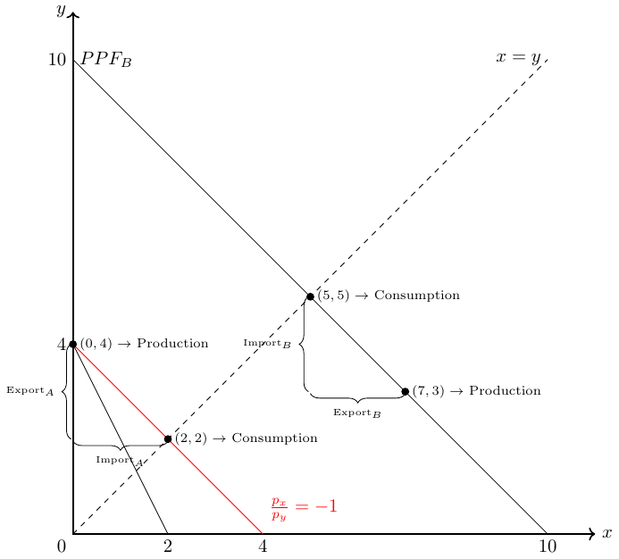
2.5.2.5 Trade structure and consumption in cooperation
If A specializes in the production of \(y\), she must import some of good \(y\), otherwise she cannot consume a bundle of both goods as desired. In turn, B wants to import some of the good \(y\). B will not accept to consume less than 5 bundles of \(y\) and \(x\) as this was his autarky consumption. Thus, B wants a minimum of 2 units of good \(y\) from A. A will not accept to give more than \(4-\frac{4}{3}=2\frac{2}{3}\) items of good \(y\) away and he wants at least \(\frac{4}{3}\) items of good \(x\). Overall, we can define three trade scenarios:
- All gains from cooperation goes to A (see Figure 2.18 and Table 2.1);
- All gains from cooperation goes to B (see Table 2.2); or
- The gains from specialization and trade are shared by A and B with a trade structure between the two extreme scenarios.
| A | B | |
|---|---|---|
| Good \(y\) | 2 | 5 |
| Good \(x\) | 2 | 5 |
| A | B | |
|---|---|---|
| Good \(y\) | -2 | 2 |
| Good \(x\) | 2 | -2 |
| A | B | |
|---|---|---|
| Good \(y\) | \(\frac{4}{3}\) | \(5\frac{2}{3}\) |
| Good \(x\) | \(\frac{4}{3}\) | \(5\frac{2}{3}\) |
| Trade | A | B |
|---|---|---|
| Good \(y\) | \(-\frac{2}{3}\) | \(\frac{2}{3}\) |
| Good \(x\) | \(\frac{4}{3}\) | \(-\frac{4}{3}\) |
Each of the three cases yield a Pareto-improvement, that is, none gets worst but at least one gets better by mutually decide on production and redistribute the joint output. In the real world, however, it is often difficult for countries to cooperate and decide mutually on production and consumption. In particular, it is practically difficult to enforce redistribution of the joint outcome so that everyone is better off. So let’s examine whether there is a mechanism that yields trade gains for both trading partners.
2.5.3 The Ricardian model
To understand the underlying logic of the argument, let us formalize and generalize the situation of two subjects and their choices for production and consumption.
In particular, the Ricardian Model build on the following assumptions:
- 2 subjects (A,B) can produce 2 goods (x,y) with
- technologies with constant returns to scale. Moreover,
- production limits are defined by \(y^i Q_y^i+ a_x^i Q_x^i=L^i\)$, where \(a^i_j\) denotes the unit of labor requirement for person \(i \in \{A,B\}\) in the production of good \(j\in \{x,y\}\) and \(Q^i_j\) denotes the quantity of good \(j\) produced by person \(i\), and \(Q^i_j\) the quantity of good \(j\) produced by person \(i\) and \(Q^i_j\) the quantity of good \(j\) produced by person \(i\). (Imagine they both work 4 hours).
- Let \(a^i_j\) denote the so-called labor input coefficients, that is, the units of labor required by a person \(i \in \{A,B\}\) to produce one unit of good \(j\in \{x,y\}\).
- Suppose further that person B requires fewer units of labor to produce both goods, that is, \(a^A_y>a^B_y\) and \(a^A_x>a^B_x\), and that
- a comparative advantage exists, that is, \(\frac{a^B_y}{a^B_x} \neq \frac{a^A_y}{a^A_x}\).
3 In order to see that the relative prices within a country equals the relative productivity parameters, consider that nominal income of labor in producing good \(j\in \{x,y\}\), \(w_jL^i_j\), must equal the production value, that is, \(p_j^ix_j^i\): \[ w_jL^i_j=p_j^ix_j^i. \] Setting \(w_j=1\) as the numeraire and re-arranging the equation, we get \[ p_j^i=\frac{L_j^i}{x_j^i}=a_j^i. \]
2.5.4 Distribution of welfare gains
The Ricardo theorem tells us nothing about the precise distribution of welfare gains. In this section, I will show that the distribution of welfare gains is the result of relative supply and demand in the world.
To illustrate this, consider Ricardo’s famous example4 of two countries (England and Portugal) that can produce cloth \(T\) and wine \(W\) with different input requirements, namely:
4 The example is explained by Suranovic (2012) in greater detail.
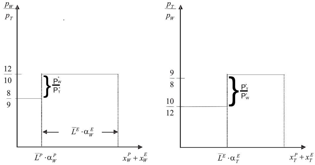
\[\begin{align*} \frac{p^P_W}{p^P_T}=\frac{a^P_W}{a^P_T}=\frac{8}{9}<\frac{12}{10}=\frac{a^E_W}{a^E_T}= \frac{p^E_W}{p^E_T} \end{align*}\] Thus, England has an absolute disadvantage in the production of both goods, but England has a comparative advantage in the production of cloth and Portugal has a comparative advantage in the production of wine. Let us further assume that both countries are similarly endowed with labor, \(\bar{L}\). Then we can calculate the world supply of cloth and wine given relative world prices, \(\frac{p_T}{p_W}\). Since we know that Portugal will only produce wine if the price of wine relative to cloth is above \(\frac{p_W}{p_T}=\frac{8}{9}\) and England will only produce wine if the price of wine relative to cloth is above \(\frac{p_W}{p_T}=\frac{12}{10}\), we can draw the relative world supply of goods as shown in the left panel of Figure 2.19. Note that \(\alpha\) in the figure means \(\frac{1}{a}\). Similarly, we can draw in the world supply of clothes, shown in the left panel of Figure 2.19.
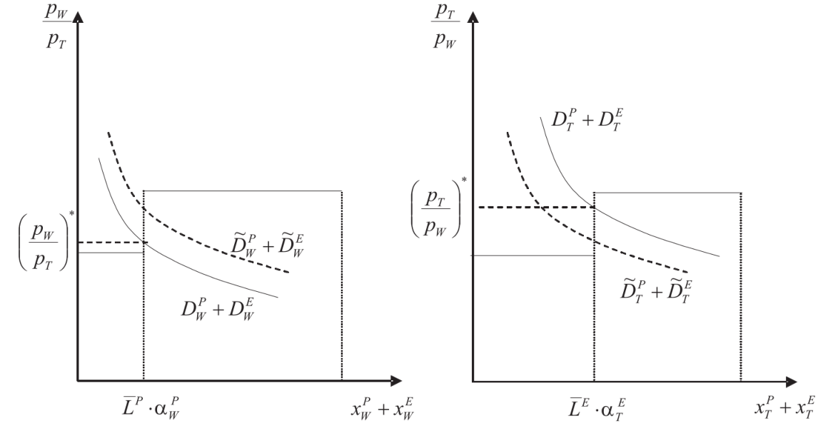
Whether both countries specialize totally in the production of one good, or only one country does so depends on world demand for both goods at relative prices. Since we know from the Ricardo Theorem that the world market price relation, \(\frac{p^{*}_T}{p^{*}_W}\), must be between the two autarky price relations: \[\begin{align}
\frac{p^P_T}{p^P_W}>\frac{p^{*}_T}{p^{*}_W}> \frac{p^E_T}{p^E_W}.
\end{align}\] If world demand for cloth would be sufficiently high to have a world price of \[\frac{p^P_T}{p^P_W}=\frac{9}{8}\] Portugal would not gain from trade. On the contrary, if world demand for wine would be sufficiently high to have a world price of \[\frac{p^P_T}{p^P_W}=\frac{10}{12}\] England would not gain from trade. Thus, the price span between \(\frac{10}{12}\) and \(\frac{9}{8}\) says us which country gains from trade. For example, at a world price of \[\frac{p^{*}_T}{p^{*}_W}=1\] about 57%
\[\begin{align}
\left[\frac{\left(1-\frac{10}{12}\right)}{\left(\frac{9}{8}-\frac{10}{12}\right)}\approx 0.57 \right]
\end{align}\] of the gains through trade will be distributed to Portugal and about 43% will be distributed to England.
In Figure 2.20, I show two demand curves of the World. The dashed demand curve represents a world with a relative strong preference on wine and the other demand curve represents a relative strong demand for cloth. Since Portugal has a comparative advantage in producing wine, they would happy to live in a world where demand for wine is relatively high, whereas the opposite holds true for England.
Exercise 2.12 Bike and tires
Consider two countries, \(A\) and \(B\). Both have a labor endowment of 24, \(L^A=L^B=24\). In both countries two goods can be produced: bikes, which are denoted by \(y\), and bike tires, which are denoted by \(x\). Assume that the two goods can only be consumed in bundles of one bike and two bike tires. The following graph illustrates the production possibility (PPF) curve of both countries in autarky, i.e, country A and B do not trade with each other.
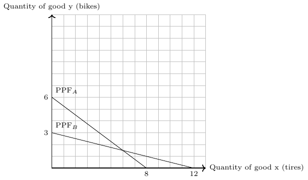
- How many complete bikes, that is, one bike with two tires, can be consumed in autarky in country A and B, respectively. Draw the production points for country A and B into the figure. (A calculation is not necessary.)
- Calculate —for both countries—the input coefficients, \(a\), that is, the units of labor needed to produce one unit of good \(y\) and good \(x\), respectively. Fill in the four input coefficients in the following table:
| Country A | Country B | |
|---|---|---|
| Good y (bikes) | (\(~~~~~~~\)) | (\(~~~~~~~\)) |
| Good x (bike tires) | (\(~~~~~~~\)) | (\(~~~~~~~\)) |
- Fill in the ten gaps (\(~~~~~~~\)) in the following text:
If we assume that both countries specialize completely in the production of the good at which they have a comparative advantage and trade is allowed and free of costs, then
country A produces (\(~~~~~~~\)) units of bikes and (\(~~~~~~~\)) units of tires and
country B produces (\(~~~~~~~\)) units of bikes and (\(~~~~~~~\)) units of tires.
Moreover, since both countries aim to consume complete bikes, that is, one bike with two tires,
country A exports (\(~~~~~~~\)) units of (\(~~~~~~~\)) and imports (\(~~~~~~~\)) units of (\(~~~~~~~\)) and
country B exports (\(~~~~~~~\)) units of (\(~~~~~~~\)) and imports (\(~~~~~~~\)) units of (\(~~~~~~~\)).
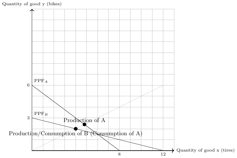
Under free trade - country A can consume (\(~~~~~~~\)) complete bikes and - country B can consume (\(~~~~~~~\)) complete bikes.
- Both countries can consume 2 complete bikes, see Figure 2.22.
| Country A | Country B | |
|---|---|---|
| Good \(y\) (bikes) | 24:6=4 | 24:3=8 |
| Good \(x\) (bike tires) | 24:8=3 | 24:12=2 |
- If we assume that both countries specialize completely in the production of the good at which they have a comparative advantage and trade is allowed and free of costs, then
- country A produces 6 units of bikes and 0 units of tires and
- country B produces 0 units of bikes and 12 units of tires.
Moreover, since both countries aim to consume complete bikes, i.e., one bike with two tires,
- country A exports 3 units of bikes and imports 6 units of tires and
- country B exports 6 units of tires and imports 3 units of bikes.
Under free trade
- country A can consume 3 complete bikes and
- country B can consume 3 complete bikes.
2.6 Trade because of different endowments (Heckscher-Ohlin model)
2.6.1 Nobel prize winning theory
The Model which we discuss in this section is named after two Swedish economist, Eli Heckscher (1879-1952) and Bertil Ohlin (1899-1979). Bertil Ohlin received the Nobel Prize in 1977 (together with James Meade). The HO-Model, as it is often abbreviated, was the main reason for the price. Here is an excerpt of the Award ceremony speech:
The Ricardo model explains international trade as advantageous because of comparative advantages that are the result of technological differences. This means that comparative advantage in the Ricardian model is solely the result of productivity differences. The size of a country or the size of the countries’ endowments does not matter for comparative advantage in the Ricardian model because there is only one factor of production in Ricardian models, namely labor. However, the assumption that there is only one factor of production is unrealistic, and we should ask what happens if there is more than one factor of production but no productivity differences? What happens if the two factors are available differently in different countries? What is the significance of endowment differences for international trade? And which owner of a factor of production will be a winner when a country opens up to world trade, and who will lose? The HO model can provide answers to these questions.
In Table 2.3, I show that countries do indeed differ substantially in their total factor productivity, capital stock, and labor endowments, which are likely correlated with total population.
| RegionCode | Capital stock at current PPPs (in mil. 2011USD) | Population (in millions) | Capital stock per capita |
|---|---|---|---|
| ITA | 10421041 | 60 | 174885 |
| ESP | 7806612 | 47 | 167518 |
| FRA | 10405968 | 65 | 160395 |
| GBR | 9973122 | 63 | 159019 |
| DEU | 12687682 | 80 | 157738 |
| USA | 48876336 | 310 | 157729 |
| AUS | 3332890 | 22 | 150382 |
| CAN | 5065392 | 34 | 148431 |
| JPN | 17161376 | 127 | 134790 |
| SAU | 3716382 | 28 | 132300 |
| KOR | 6052155 | 49 | 123287 |
| TWN | 2835890 | 23 | 122549 |
| ROU | 1271652 | 20 | 62647 |
| VEN | 1765996 | 29 | 60905 |
| BRA | 9869311 | 199 | 49691 |
| RUS | 6746460 | 143 | 47126 |
| POL | 1769004 | 39 | 45859 |
| THA | 2977965 | 67 | 44652 |
| IRN | 3234132 | 74 | 43555 |
| ARG | 1773984 | 41 | 43034 |
| MEX | 5054693 | 119 | 42613 |
| TUR | 2938288 | 72 | 40634 |
| UKR | 1616826 | 46 | 35420 |
| IDN | 8146254 | 242 | 33716 |
| COL | 1446480 | 46 | 31501 |
| CHN | 42218080 | 1341 | 31483 |
| PER | 681036 | 29 | 23185 |
| PHL | 1560017 | 93 | 16767 |
| IRQ | 443733 | 31 | 14375 |
| IND | 15356803 | 1231 | 12475 |
Source: Penn World Tables 9.0
2.6.2 The Heckscher-Ohlin (factor proportions) model
Assumptions:
Two countries: Home country and foreign country. Variables referring to foreign countries are marked with an asterisk, \(*\).
Two goods: \(x\) and \(y\).
Two factors of production: \(K\) and \(L\). This is new in relation to the Ricarkian model! Let’s name the factors \(K\) and \(L\), which stands for capital and labor.
Goods differ in terms of their need for factors of production: \[\frac{K_y}{L_y} \neq \frac{K_x}{L_x}.\] This means that one good must be produced in a capital-intensive way and the other in a labor-intensive way. If we assume that good \(y\) is capital intensive and good \(x\) is labor intensive in production, we can write: \[\begin{align*} \frac{K_y}{L_y} > \frac{K_x}{L_x}. \end{align*}\] In this inequality, the quantity of capital required to produce good \(y\), \(K_y\), is on the left-hand side relative to the quantity of labor required to produce good \(y\), \(L_y\), that is, the capital intensity of good \(y\).The capital intensity of good \(x\) is on the right-hand side of the inequality. Rewriting this inequality, we can express it in terms of labor intensities: \(\frac{L_y}{K_y} < \frac{L_x}{K_x}.\) It should be clear that both inequalities say the same thing.
No technology differences between countries: Since we already know from Ricardian theory that productivity or technology differences are a source of international trade, we do not want to explain the same thing again with the HO model. So we assume that all input coefficients are the same in all countries.
Different relative factor endowments: \[\frac{K}{L} \neq \frac{K^*}{L^*}.\] Since countries are assumed to have different factor endowments, the model links a country’s trade pattern to its endowment of factors of production. The capital-labor ratio in the home country, \(\frac{K}{L}\), must differ from the ratio abroad. Suppose the home country is capital-rich and the foreign country is labor-rich. Then we have the following ratios between capital and labor in the two countries: \[\begin{align*} \frac{K}{L} > \frac{K^*}{L^*}. \end{align*}\] This means that the capital-labor ratio (a country’s capital intensity) is higher in the home country than abroad. In terms of the ratio between labor and capital, that is, the labor intensity of a country, this can be expressed as follows: \(\frac{L}{K} < \frac{L^*}{K^*}.\) It should be clear that both inequalities say the same thing.
Free factor movement between sectors Both factors can be used in the production of both goods. Note that cross-country movement of factors (migration, foreign direct investment) is not allowed.
No trade costs Final products can be traded without any costs.
Equal tastes in countries and homothetic preferences Consumers in both countries have the same utility function. Homothetic preferences simply mean that for given relative prices, income does not affect the ratio of consumption.
2.6.3 Heckscher-Ohlin theorem
- Consider that the home country has relatively more capital and the foreign country relatively more labor and that the good \(y\) is capital intensive in production whereas the good \(x\) is labor intensive.
- Then it is relatively cheap for the home country to produce the capital-intensive good because it is endowed with a lot of capital, while it is relatively costly to produce the good with which the country is hardly endowed.
- Thus, the home country has a comparative advantage in producing the capital-intensive good.
- The opposite is true for the foreign country.
2.6.4 Factor-price equalization theorem
- As a result of the Heckscher-Ohlin theorem, output of the good in which the country has a comparative advantage would increase. The capital intensive country will produce more capital intensive goods and the labor intensive country will produce more labor intensive goods.
- As the production of the good that makes intensive use of the abundant resource increases, the demand for that resource will also increase. Demand for the scarce resource will also increase, but to a lesser extent.
- If production of the good that intensively uses the scarce resource decreases, both abundant and scarce resources will be released, but relatively more of the scarce resource than of the abundant resource.
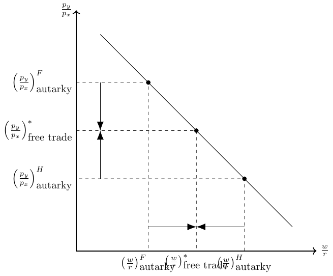
- In autarky, the relatively scarce factor in the home country was labor and factor prices were as follows: \[ \frac{w}{r}>\frac{w^*}{r^*} \]
- After opening to trade, production shifts to the home country so that the wage falls (\(w\downarrow\)) and the rent rises (\(r\uparrow\)).
- After opening to trade, production shifts abroad so that the wage rises, \(w^*\uparrow\), and the rent falls, \(w^*\downarrow\).
- This reallocation process, and hence the change in factor prices, continues until factor prices are equal in all countries: \[
\frac{w}{r}=\frac{w^*}{r^*}
\]
- Figure 2.23 visualizes the reasoning behind the factor-price equalization theorem.
- I recommend a clip of Mike Moore explaining how trade based on factor endowments affects wages and returns to capital, see this video:
Why does the Factor-Price Equalization Theorem not (fully) hold?
In the real world, factor prices do not equalize due to frictions such as transportation costs, trade barriers, and the presence of goods that are rarely or never traded.
Trade as an alternative to factor movements:
The factor price equalization theorem contains an interesting insight: if a country allows free trade in its products, it will automatically export the abundant factor indirectly in the form of goods that intensively use the abundant factor.
Exercise 2.15 HO-Model in one figure
Suppose consumers from country A and the foreign country B like to consume two goods that are neither perfect substitutes nor perfect complements. Moreover, assume for simplicity that both countries have the same size but have different endowments, as stated in the assumptions above. Moreover, assume the factor intensity of production as stated in the assumptions above.
- Sketch the production frontiers for both countries in autarky. Show graphically the relative price in autarky.
- You will see that the relative prices of goods differ across countries: \[\begin{align*} \left(\frac{p_1}{p_2}\right)\neq\left(\frac{p_1}{p_2}\right)^*. \end{align*}\] That means, the Home country A has a comparative advantage in producing good \(1\).
- Now, sketch the world market price that will maximize the utility.
- Where are the new production and consumption points of both countries?
- Show in the graphic how much each country trades.
- I recommend a clip of Mike Moore who also explains the HO-Model with production possibility curves, see this video.
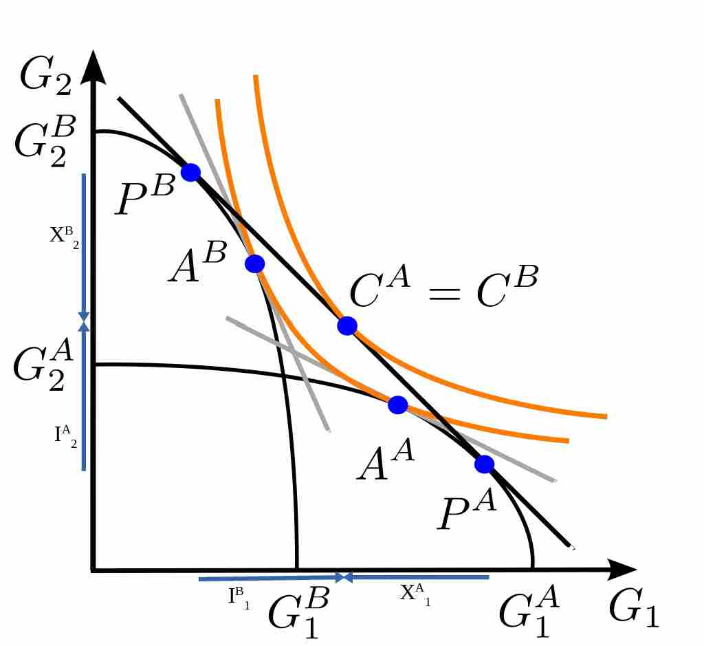
Two identical countries (A and B) have different initial factor endowments. I assume that country A is abundantly endowed with the production factor that is intensively used in the production of good 1, the reverse holds for country B. Thus, the two solid black lines in Figure 2.24 represents the respective production possibility frontier curves. The orange lines represents the respective indifference curves. Autarky equilibria are marked with \(A^{A}\) and \(A^{B}\), respectively. The production points in trade equilibrium are marked with \(P^A\) and \(P^B\), the consumption point of both countries is in \(C^A=C^B\). Thus, production and consumption points are divergent. The indifference curve under free trade is clearly above the other indifference curve in autarky. The solid black line that is tangient to the consumption point under free trade represents the utility maximizing world market price under free trade. The exports, \(X\), and imports; \(I\), are denotes correspondingly to the goods and country names.
2.7 The specific factor model
Source: otherwords.org
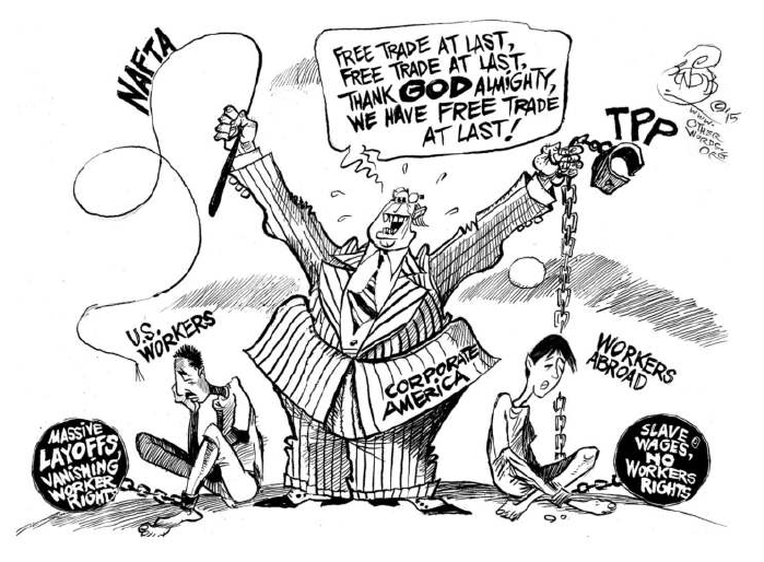
From the Ricardian model, we know that trade is a positive-sum game. If free trade is beneficial to a country, as Ricardo predicts, why isn’t everyone happy with free trade? In democratic societies, policymakers sometimes adopt protectionist trade policies because of pressure from interest groups and public demand. The discrepancy between the promises and potential benefits of trade on the one hand and the negative consequences of free trade for many groups on the other is illustrated in Figure 2.25. The models so far do not give us a way to see which groups actually suffer from free trade, and thus we have no clue why there are incentives for interest groups to oppose free trade. Are anti-free trade policy preferences the result of ignorance, general worldviews, political ideology, environmental attitudes, social trust, or other factors? Well, these things may play a role, but there are also economic factors, that is, the self-interest of individuals and groups within an economy, that can account for anti-free trade attitudes. In the following sections, we will discuss a theory that shows that while free trade benefits countries as a whole, not everyone within a country benefits equally. Some benefit more than others, and some are actually made worse off by free trade.
In the next two subsections, we derive some key hypotheses that free trade favors those people in a country who have abundant factors of production and disadvantages those who have scarce factors. Moreover, free trade favors investors and workers in export-oriented industries with comparative advantages.
2.7.0.1 Assumptions
The sector-specific model, also known as the Ricard-Viner model, can show that there are winners and losers in international trade. The model is based on the following assumptions:
- 2 countries \(i \in \{A, B\}\)
- 2 goods (sectors) \(g \in \{1, 2\}\)
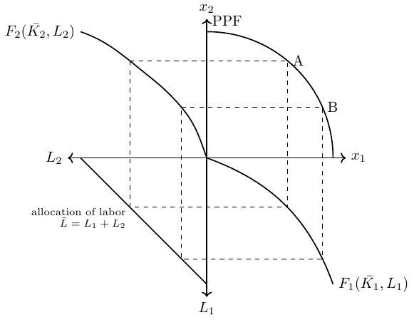
- 3 factors of production: Labor \(L\), capital specific to the production of good 1, \(K_1\), and capital specific to the production of good 2, \(K_2\)5. The technologies for the production of both goods are now represented by two production functions \(Q_1=F_1(\bar{K_1},L_1)\) and \(Q_2=F_2(\bar{K_2},L_2)\), where both factors of production have positive but decreasing marginal products
- The capital allocated to each sector is fixed for both countries: \(K_1=\bar{K}_{1}, K_2=\bar{K}_{2}\)
- The labor assigned to each sector (\(L_1\) and \(L_2\)) can change in response to external shocks: \(\bar{L}=L_1+L_2\)
- perfect competition
- perfect market clearing (no unemployment)
- country A is a small open economy (we consider only country A and therefore do not use a subscript for countries in the following)
5 You can think of capital specific to the production of manufacturing goods (good 1) and land specific to the production of food sector goods (good 2)
2.7.0.2 The production possibility frontier with two factor inputs:
The two production functions, the fixed endowments and the distribution of labor determine the aggregate PPF. The PPF, which is the product of two production functions (\(F_1\) and \(F_2\)), is shown in Figure 2.26. The figure shows, for both production points A and B, how the mobile factor of production, labor, must be reallocated from sector 2 to sector 1 in order to produce more of good 1 in production point B. The second and fourth quadrants show the respective production functions of sectors 1 and 2.
2.7.0.3 Equillibrium in autarky:
- Depending on a country’s demand for good 1 and 2 a production point on the PPF is chosen at which it must hold that the slope of the PPF curve and the price relation (that is, relation of marginal product of labor in sector 1 and sector 2) must be equal: \[\begin{align*} \frac{p_1}{p_2}=\frac{\frac{\partial F_2}{\partial L_2}}{\frac{\partial F_1}{\partial L_1}} \end{align*}\]
- What can we say about the rents of the production factors?
- From the assumption of perfect competition it follows that firms do not make a positive profit in equilibrium, \(\pi\overset{!}{=}0\). Thus, the equilibrium wage for sectors \(g \in \{1, 2\}\) are given by the profit maximizing of firms \[\begin{align*} \pi_g&=p_g\cdot F_g(\bar{K_g},L_g)-w_gL_g-r_gK_g\\ \frac{\partial \pi_g}{\partial L_g}&= p_g\cdot \frac{\partial F_g}{\partial L_g}-w_g\overset{!}{=}0 \qquad \Leftrightarrow w_g=p_g\frac{\partial F_g}{\partial L_g} \end{align*}\]
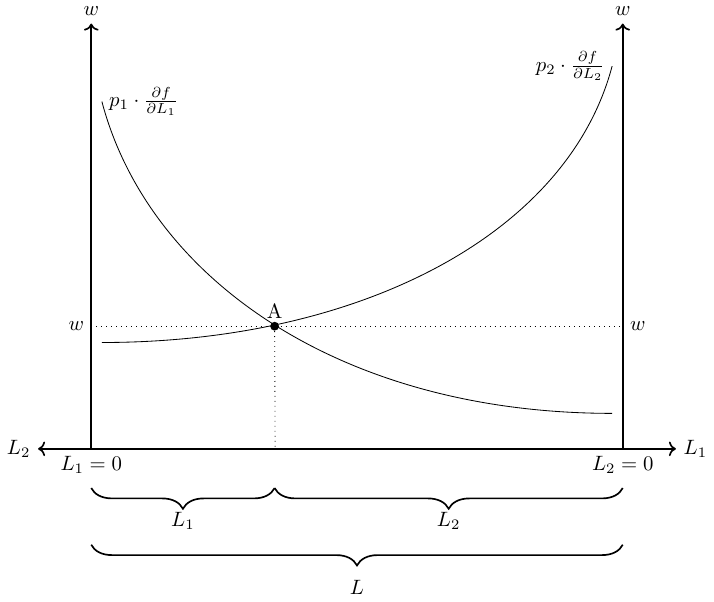
- We know that labor can move freely between sectors and an equilibrium exists when there are no incentives to move any further. That is the case when wages in both sectors are equal, \(w_1=w_2\). Thus, we can express wages in terms of purchasing power in units of good 1 as follows: \[\begin{align*} w_1&=p_1\frac{\partial F_1}{\partial L_1}\qquad \text{ and } \qquad w_2=p_2\frac{\partial F_2}{\partial L_2}\\ \Rightarrow w&=p_1\frac{\partial F_1}{\partial L_1}=p_2\frac{\partial F_2}{\partial L_2}\\ \Leftrightarrow \frac{w}{p_1}&=\frac{\partial F_1}{\partial L_1}\\ \Leftrightarrow \frac{w}{p_2}&=\frac{\partial F_2}{\partial L_2} \end{align*}\]
- Figure 2.27 presents the equilibrium wage and the optimal allocation of labor into sector 1 and 2.
2.7.0.4 Equilibrium under free trade:
Assume the price of good 1 and good 2 increase due to a trade opening in the same proportion. What happens with the real wage and the real incomes of capital-1 and capital-2 owners? The answer is: no real changes occur.
- The wage rate, \(w\), rises in the same proportion as the prices, so the real wages are unaffected. In Figure 2.27 this can be shown by shifting both curves upward.
- The real incomes of capital owners also remain the same because there will be no reallocation of labor across sectors.
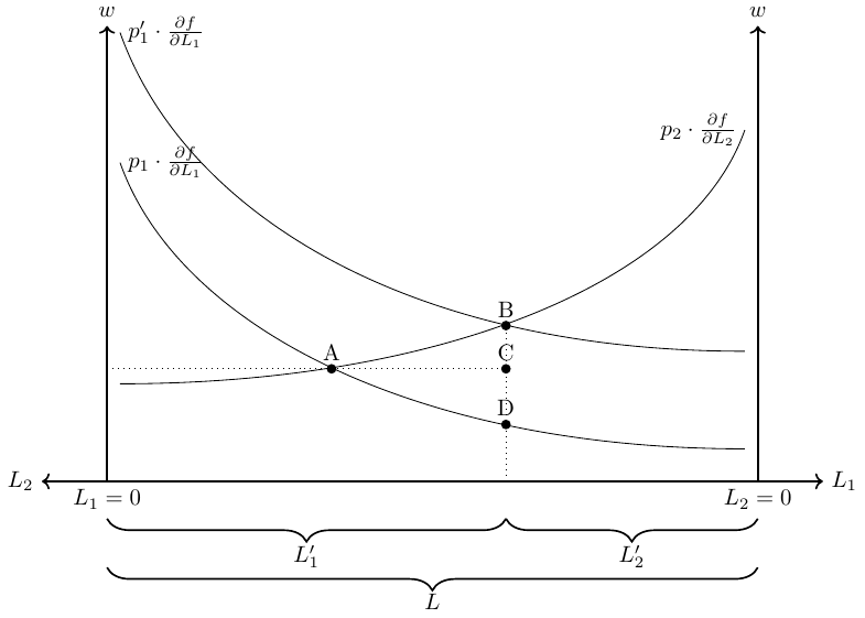
Now, assume only the price of good 1 rises for 10% while \(p_2\) remains fixed, \(\frac{p'_1}{p_2}>\frac{p_1}{p_2}\). What happens with the real wage and the real incomes of capital-1 and capital-2 owners? The answer is: some win, some lose, and some maybe win.
2.7.0.5 Wages:
- \(p_1\frac{\partial F_1}{\partial L_1}\) rises and hence labor reallocates from sector 2 to sector 1 (\(L_1\uparrow\) and \(L_2\downarrow\)). This is shown in Figure 2.28.
- This reallocation of labor has some implications for the real wages measured in purchasing power of good 1 and 2, respectively:
- The price of good 1 has increased by 10%, the wage has however increased by less than 10% (compare the length of BC and BD in the figure), whereas the price for food stays constant.
- Thus, the purchasing power in buying good 2 increased, whereas the purchasing power in buying good 1 decreased. Hence, workers gain when buying good 2 but lose when buying good 1
- Overall, the welfare effect from real wages is unclear and depends on preferences.
2.7.0.6 Owner of capital-1:
- Owners of capital-1 receive a 10% higher price on their products but have to pay a less than 10% higher wage.
- Overall, capital-1 owners gain from free trade because they can employ more workers (at a higher price) now.
2.7.0.7 Owner of capital-2:
- Owner of capital-2 receive the same price on their products but have to pay a higher wage.
- Overall, capital-2 owners lose from free trade because they can employ less workers at a higher price now.