1 Monetary international economics
1.1 Currencies
An exchange rate indicates the value of one currency in relation to another. Exchange rate fluctuations have a significant impact on the revenues, costs, and profits of businesses; they affect how much you can afford to spend and can even influence job security.
Please work on the questions posed in Exercise 1.1 and Exercise 1.2. They are designed to motivate an introduction the topic.
Exercise 1.1 Exchange rates over time
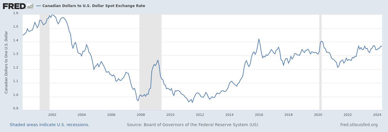
- As can be seen in Figure 1.1, 1 United States Dollar (USD) equals about 1.38 Canadian Dollar (CAD) today. Since January 2002, has the USD depreciated (lost value) or appreciated (gained value) against the CAD? Explain your decision.
- Assume that in January 2002, you exchanged a total of 2000 USD to Canadian Dollars (CAD) at a rate of 1.6 CAD per USD. Calculate how much that amount is worth today in USD.
Suppose you have 1000 USD today, that is January 2024, and you plan to invest it in a Canadian fund that assures you a 2% annual interest rate.
- Calculate how much USD you’ll have after one year if the exchange rate remains on its current level of 1.38 CAD per USD.
- Calculate how much USD you’ll have after one year if the exchange rate slightly chances to 1.42 CAD per USD.
Exercise 1.2 Our relations are not good
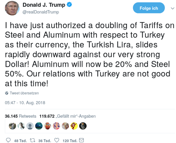
Source: Twitter
Why is Trump implicitly expressing concerns about the weak Lira and the strong Dollar? Would he prefer a “strong” Turkish Lira and a “weak” Dollar? What factors actually contribute to his satisfaction? Can you understand the logic behind President Trump’s decision to double metal tariffs in response to the decline of the Turkish Lira (see Figure 1.2)? Discuss.
1.1.1 Exchange rates
The most important economic indicators frequently discussed in the media and politics are Gross Domestic Product (GDP)1, the policy rate2, and the inflation rate3. These measures are designed to explain the functioning of economic markets and guide policymakers. However, the exchange rate is used less frequently in political and public debates, which I believe is a significant oversight for several reasons.
1 The total value added of a country in a given period
2 The interest rate set by a central bank that influences the lending and borrowing rates of commercial banks to control inflation, manage employment levels, and stabilize the currency
3 The percentage increase in the general price level of goods and services in an economy over a given period
Firstly, similar to the aforementioned measures, exchange rate movements have a substantial impact on both markets and individuals. Moreover, the exchange rate serves as an accurate measure that reflects real market movements more quickly than most other indicators. Overall, a solid understanding of exchange rates is crucial for making informed decisions, managing financial risks, optimizing operations, and strategically positioning companies in the global marketplace.
Before I explain this in greater detail, let me share my explanations for why the exchange rate is relatively unnoticed in public debates:
- Complexity of interpretation: It is comparatively difficult to interpret. GDP should be rising, while the inflation and policy rates should ideally be low. In contrast, the exchange rate is not so straightforward because there isn’t a universally optimal exchange rate that everyone hopes for. The ideal rate depends on many factors, such as whether you want to buy goods from abroad or sell them to the rest of the world. Different stakeholders and investors will have varying preferences about the exchange rate. Many people, especially politicians, avoid the complexities of “it depends” arguments because it is challenging to make convincing cases based on intricate relationships.
- Volatility: The exchange rate is comparatively volatile, and its changes are difficult to predict.
- Multiple exchange rates: There isn’t just one exchange rate; there are many, as any currency can be exchanged for any other currency. This means that a country’s exchange rate may rise against currency A but fall against currency B.
- Limited political influence: The power of politics to directly and measurably influence a country’s exchange rate is limited.
- Understanding requirements: The impact of exchange rate movements on our lives requires a solid understanding of economic markets, which many people lack.
While I cannot change the factors that contribute to the limited discussion of exchange rates, I can work to help you make sense of this topic. Before discussing the importance of the exchange rate in Section 1.1.3, let’s first define the rate:
The price of one currency in terms of another is called an exchange rate. Exchange rates allow us to compare the prices of goods and services across countries, determining a country’s relative prices for exports and imports.
To define the rate more formally, suppose the Euro (€) is the home currency and Turkish Lira (₺) the foreign currency, then the exchange rate in direct quotation (Preisnotierung) is \[E^{\frac{\text{€}}{\text{₺}}}=\frac{X \text{€}}{Y \text{₺}}\] and the exchange rate in indirect quotation (Mengennotierung) is \[E^{\frac{\text{₺}}{\text{€}}}=\frac{Y \text{₺}}{X \text{€}}.\]
Both rates contain the same information, but have different interpretations:
- \(E^{\frac{\text{€}}{\text{₺}}}\) tells that we have to give X to receive Y , whereas
- \(E^{\frac{\text{₺}}{\text{€}}}\) tells that we have to give Y to receive X .
Alternative interpretations:
- \(E^{\frac{\text{€}}{\text{₺}}}\) tells that we have to give \(\frac{X}{Y} \text{€}\) to receive 1 , whereas
- \(E^{\frac{\text{₺}}{\text{€}}}\) tells that we have to give \(\frac{Y}{X} \text{₺}\) to receive 1 .
A currency can appreciate or depreciate relative to other currencies.
- If the appreciates, \(E^{\frac{\text{€}}{\text{₺}}}\) decreases and \(E^{\frac{\text{₺}}{\text{€}}}\) increases.
- If the depreciates, \(E^{\frac{\text{€}}{\text{₺}}}\) increases and \(E^{\frac{\text{₺}}{\text{€}}}\) decreases.
- Euro to Dollar means \(\frac{\text{€}}{\$}\) (This is especially confusing and it can also be understood the other way round but the first currency mentioned is usually interpreted as the numerator)
- Euro per Dollar means \(\frac{\text{€}}{\$}\)
- Euro in Dollar means \(\frac{\$}{\text{€}}\)
- 1 Euro costs X Dollars means X \(\frac{\$}{\text{€}}\)
Exercise 1.3 Interpret the exchange rate representations shown in Figure 1.3. Consider the Euro as the home currency and write the most recent currency rates of the four figures in direct quotation.

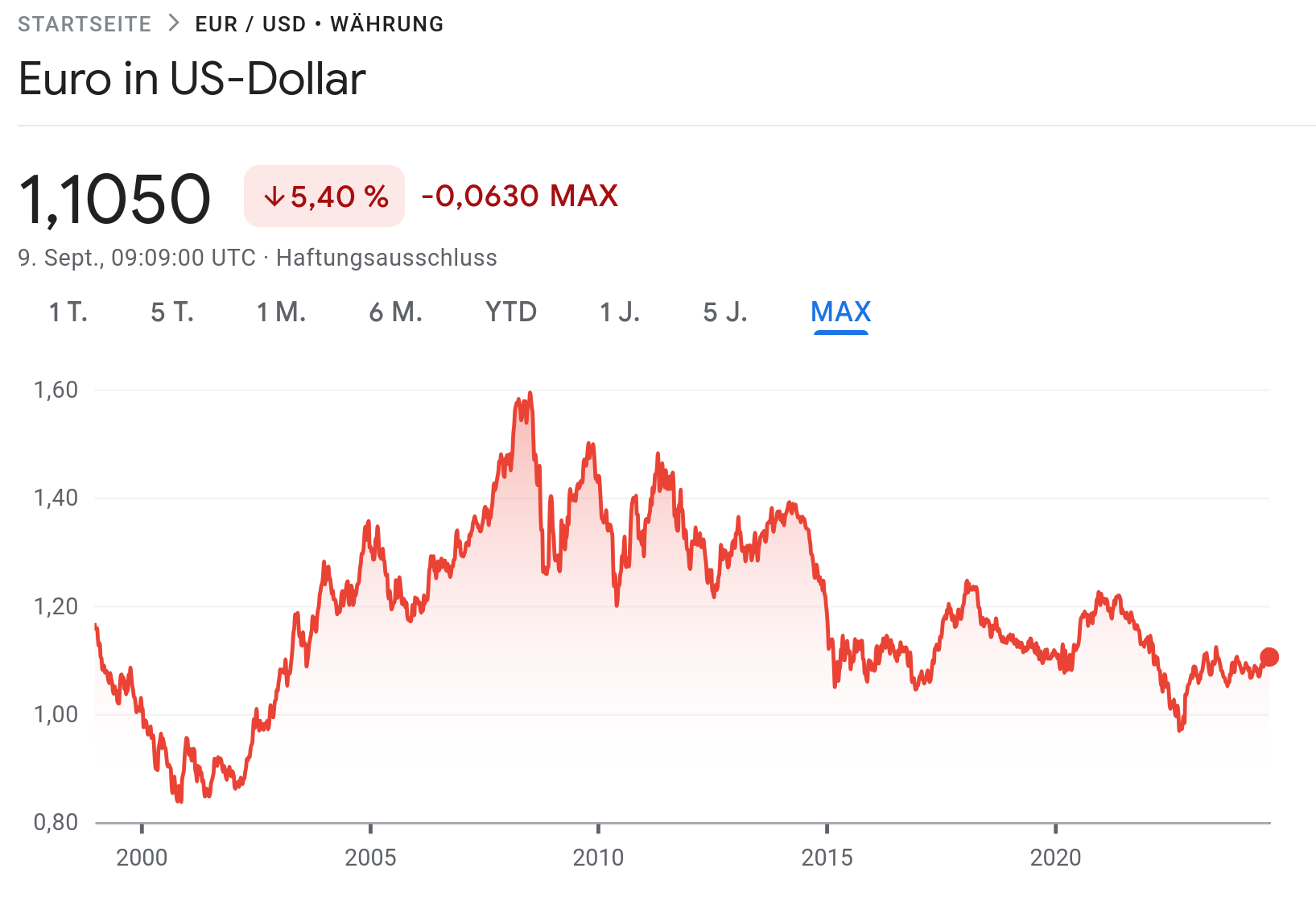
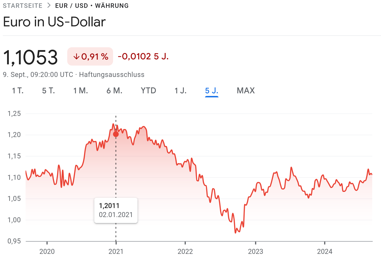
Source: Subfigures (c) and (d) are taken from Google.
1.1.2 Relative prices and exchange rates
After understanding the concept of exchange rates, let us consider how trade in goods between two countries operates when each country uses a different currency as its legal tender.
Let us consider a stylized example: Assume the home country produces beer and the foreign country produces wine. If you want to exchange a beer for wine, the relative price indicates the amount of beer you need to provide in order to receive a unit of wine (in direct quotation) or the quantity of wine you will receive for a unit of beer (in indirect quotation).
For example, a relative price of 1 means you can exchange 1 liter of beer for 1 liter of wine. However, if we assume that beer is measured in 500 ml cans and wine in 1-liter bottles, the relative price denoted with \(P^{\frac{beer}{wine}}\) would be represented as:
\[P^{\frac{beer}{wine}}= \frac{2 \text{ cans of beer}}{1 \text{ bottle of wine}}.\]
This means you can exchange 2 cans of beer for one bottle of wine.
If the relative price increases, you will need to provide more beer to receive a bottle of wine. Conversely, if the relative price decreases, you will need to provide less beer to obtain a bottle of wine.
Relative prices determine the relative price of commodities across countries. For example, an increase in the price of foreign commodities makes imported commodities relatively more expensive and home commodities relatively cheaper for buyers at home.
Relative prices are (directly) determined by exchange rates. To logically prove this statement, let us assume for simplicity an exchange rate of 1, \[E^{\frac{\text{₺}}{\text{€}}}=E^{\frac{\text{€}}{\text{₺}}}=1\] and that a liter of beer costs 1 € at home and a wine costs 1 ₺ abroad. Thus, we can buy both a wine or a beer for 1 €. Due to the fact that we must pay the wine producer with ₺, we must convert the € beforehand. The process goes like visualized in Figure 1.4:

Now, assume that the € appreciates and the exchange rate becomes \(E^{\frac{\text{€}}{\text{₺}}}=0.5\) and \(E^{\frac{\text{₺}}{\text{€}}}=2\), respectively. Then, you receive more than one wine if we assume that the price of wine in ₺ remains unchanged. The process is visualized in Figure 1.5:

That means, exchange rates determine the relative prices. If the home currency appreciates (depreciates), buying goods and services abroad becomes relative cheaper (more expensive).
Of course, if many people now buy wine and aim to convert € to ₺, this may impact the exchange rate and the price of wine. We come back to that later.
The exchange rate determines the relative price of commodities across countries. For example, an appreciation of a currency makes commodities more expensive for foreign buyers and in turn makes foreign commodities cheaper for buyers at home.
1.1.3 The importance of exchange rates
Here is an incomplete list of arguments to emphasize the importance of exchange rates for economies, businesses, and individuals:
- Import/export costs: Exchange rate fluctuations determine the relative prices and hence affect the cost of importing goods and materials and the global demand for domestic products. An appreciation of the home currency makes imports relatively cheaper but exports more expensive for the rest of the world, while depreciation has the opposite effect.
- Revenue conversion: Multinational companies earn revenues in multiple currencies. Exchange rate changes can significantly impact the value of these revenues when converted back to the home currency, affecting overall profitability.
- Foreign investments: Companies investing in foreign assets or operations need to understand exchange rates to forecast returns accurately and manage exchange rate risk.
- Risk management: Knowledge of exchange rates enables businesses to hedge against currency risk using financial instruments like forwards, futures, options, and swaps. This is crucial for stabilizing cash flows and protecting profit margins.
- Market competitiveness: Exchange rates affect the relative cost competitiveness of goods and services in international markets. Companies need to understand these implications to price their products competitively and make strategic decisions about entering or exiting markets.
- Macroeconomic insights: Exchange rates are influenced by and also affect economic indicators such as inflation, interest rates, and economic growth. Understanding these relationships helps in making informed predictions about market conditions.
- Contractual agreements: Businesses engaged in international trade must understand exchange rates to negotiate and structure contracts effectively, determining terms such as the currency of payment and exchange rate clauses.
- Government and Policy Understanding: Exchange rates are often influenced by governmental and central bank policies. Understanding the dynamics between exchange rates and policy decisions is vital for anticipating regulatory changes and their potential impact on business operations.
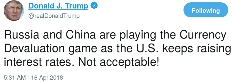
1.1.4 Trump, relative prices, and trade policy
Let’s return to Trump’s Twitter message . Steel producers in the U.S. (and Donald Trump himself) are unhappy about a strong dollar (and a weak Turkish Lira) because it makes their products relatively expensive for Turkish buyers while making Turkish steel relatively cheap for U.S. consumers.
Trump had two options to address this issue: altering the exchange rates or adjusting the relative prices of goods between countries. Changing the exchange rate directly is a challenging task. Although buying or selling currencies on the foreign exchange market can influence exchange rates, the market is so large that the actions Trump could take as President would have minimal impact (see Section 1.1.5). Adjusting policy rates could influence exchange rates more effectively, as we will discuss in Section 1.2. However, the Federal Reserve, which sets policy rates and thus has an impact on interest rates, operates independently from political orders. Consequently, Trump’s influence over their decisions is limited.
As a result, Trump chose to increase the price of foreign steel in the U.S. by introducing or raising tariffs. The approach works, American steel producing companies get protected from foreign competition and might sell more domestically. However, there many negative consequences that detoriate the overall welfare. Foremost, everybody in the U.S. must pay more for steel (and for products made with steel and aluminum). David Boaz, Executive Vice President of the Cato Institute, a libertarian think tank, highlights this issue in his response on Twitter (see Figure 1.6).

Source: Twitter
To quantify the costs of Mr. Trumps’s tariffs, let me quote the well-written article by Amiti et al. (2019) (p. 188-189):
In addition, it can be argued that increased tariffs might actually make the dollar stronger. If buyers stop purchasing steel from Turkey due to higher tariffs, they will need fewer Turkish lira and therefore will exchange fewer U.S. dollars for Turkish lira. This reduced demand for Turkish lira could lead to a stronger dollar.
While raising tariffs and initiating trade disputes could be a strategy to gain political support and possibly get re-elected, there is a general consensus among economists that raising tariffs usually leads to economic losses and detrimental outcomes for all countries involved.
1.1.5 The FOREX
1.1.5.1 The market
In a market, individuals exchange goods and services, offering something to receive something else in return. In the FOREX (foreign exchange market), participants exchange currencies. Like all markets, the price here is influenced by the supply and demand dynamics of currencies.
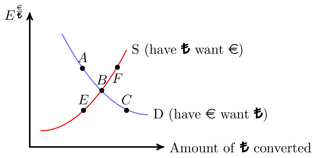
- When the Euro (€) is considered strong, the exchange rate \(E^{\frac{\text{€}}{\text{₺}}}\) is low:
- At this lower exchange rate, there’s a high demand for Turkish Lira (₺) (point C), but the supply of ₺ is scarce (point E).
- Consequently, the Euro faces depreciation pressure, leading to an increase in the exchange rate \(E^{\frac{\text{€}}{\text{₺}}} \uparrow\).
- Conversely, when the Euro (€) is weak, the exchange rate \(E^{\frac{\text{€}}{\text{₺}}}\) is high:
- With the exchange rate high, the demand for ₺ drops (point A), while its supply burgeons (point F).
- As a result, the Euro is under appreciation pressure, causing the exchange rate to decrease \(E^{\frac{\text{€}}{\text{₺}}} \downarrow\).
- Point B represents the equilibrium exchange rate, where the demand for ₺ meets its supply. At this juncture, holders of ₺ are unwilling to part with more, and similarly, Euro holders are not inclined to exchange more.
In 2022, the daily (!) traded volume of currencies averaged approximately $ 7,506 billion, as highlighted in Table 1.1.
| name | 2001 | 2004 | 2007 | 2010 | 2013 | 2016 | 2019 | 2022 |
|---|---|---|---|---|---|---|---|---|
| Total | 1.239 | 1.934 | 3.324 | 3.973 | 5.357 | 5.066 | 6.581 | 7.506 |
| USD | 1.114 | 1.702 | 2.845 | 3.371 | 4.662 | 4.437 | 5.811 | 6.639 |
| EUR | 470 | 724 | 1.231 | 1.551 | 1.790 | 1.590 | 2.126 | 2.292 |
| JPY | 292 | 403 | 573 | 754 | 1.235 | 1.096 | 1.108 | 1.253 |
| GBP | 162 | 319 | 494 | 512 | 633 | 649 | 843 | 968 |
| CNY | 0 | 2 | 15 | 34 | 120 | 202 | 285 | 526 |
| AUD | 54 | 116 | 220 | 301 | 463 | 349 | 446 | 479 |
| CAD | 56 | 81 | 143 | 210 | 244 | 260 | 332 | 466 |
| CHF | 74 | 117 | 227 | 250 | 276 | 243 | 326 | 390 |
| All others combined | 170 | 251 | 568 | 786 | 1124 | 1223 | 1921 | 2093 |
Note: All others combined are: HKD, SGD, SEK, KRW, NOK, NZD, INR, MXN, TWD, ZAR, BRL, DKK, PLN, THB, ILS, IDR, CZK, AED, TRY, HUF, CLP, SAR, PHP, MYR.
Source: https://github.com/TheEconomist/big-mac-data (July 18, 2018).
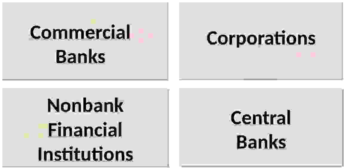
1.1.5.2 Actors on the FOREX
As indicated in Figure 1.8, there are several major players involved in trading on the foreign exchange market. In particular, commercial banks, multinational corporations and non-bank financial institutions, such as investment funds, play an important role in trading and speculation. Central banks also play a crucial role as they intervene to stabilize their national currency and thus influence the direction of the market.
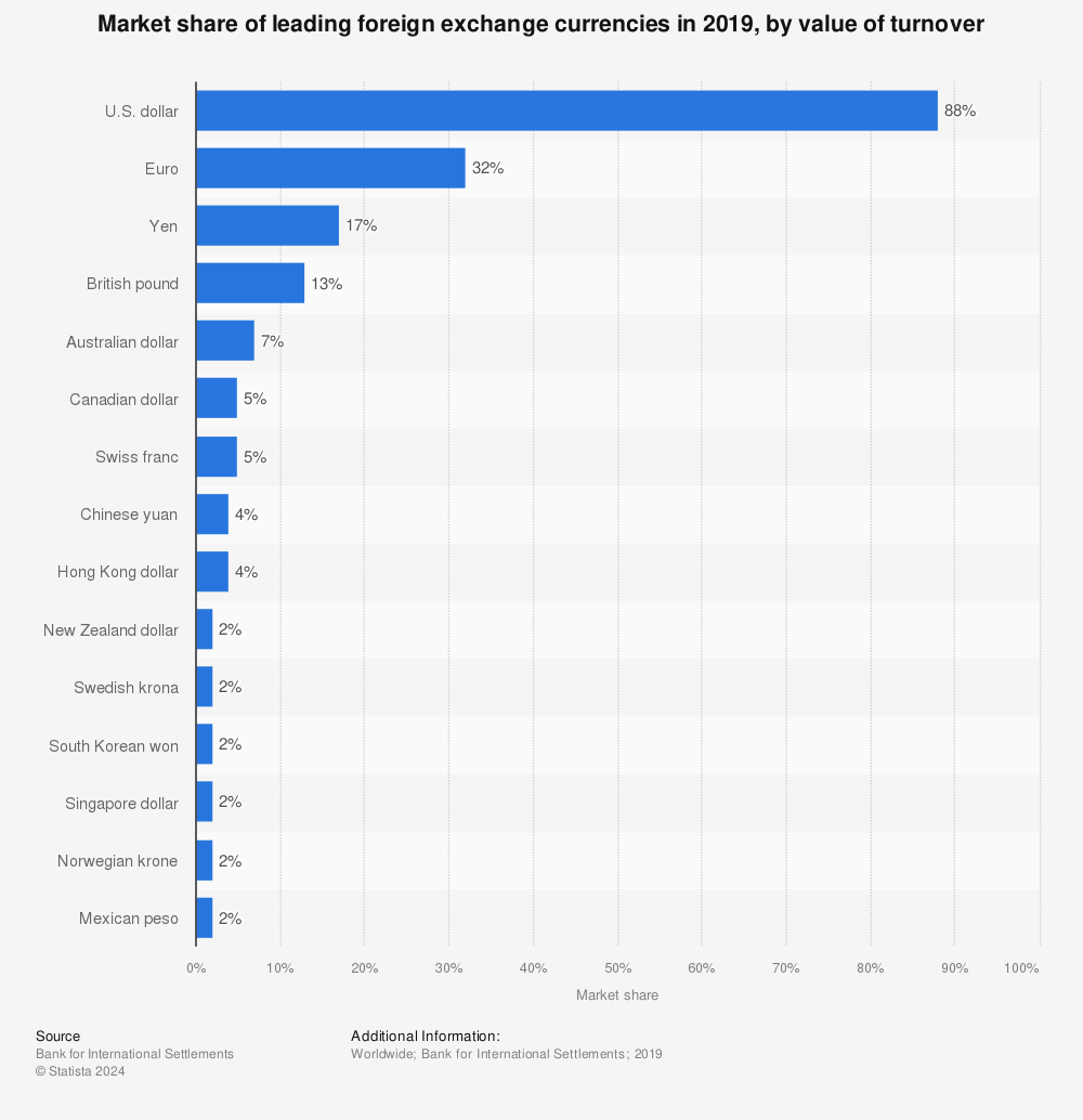
1.1.5.3 The vehicle currency
Instead of converting directly between two less common currencies, it’s more efficient to use a broadly accepted and stable currency as a vehicle. That means, if you want to exchange currency A to B. You do not exchange currency A directly to B but you convert currency A first to the vehicle currency C and then from C to B.
As depicted in Figure 1.9, around 32% of all currency transactions included the Euro while a notable 88% involved the U.S. Dollar which makes the Dollar the standard vehicle currency. The Dollar acts as a medium in transactions between currencies that do not directly trade with high volume. This can reduce transaction costs and streamline the process.
1.1.6 Purchasing power parity assumption
The Purchasing Power Parity (PPP) assumption is also know as the law of one price. It says that in competitive markets with zero transportation costs and no trade barriers, identical goods have the same price all over the world when expressed in terms of the same currency. The idea behind this is that if differences in prices exist, profits can be made through international arbitrage, that is, the process of buying a good cheap in one country and selling the good with a profit in another country. This process can quickly equalize real price differences across countries.
However, in the real world, prices differ substantially across countries (see the Big Mac Index in Table 1.2 and Exercise 1.5). The assumptions of the PPP do mostly not hold perfectly in reality: some goods and services are not trade-able, firms might have different degrees of market power across countries, and the transaction costs are not zero. Here are more reasons, why the PPP does not always apply, especially in the short run:
- Transportation costs are not zero. Shipping goods can be time consuming and expensive.
- Many goods and services, such as real estate or personal services, cannot be traded.
- International markets may be segmented due to regulatory barriers, tariffs and other trade restrictions.
- Countries have different consumption preferences. That means, the same basket of goods is not necessarily equally demanded. The willingness to pay for goods vary across countries often significantly.
- Countries impose different taxes and provide different subsidies on goods and services, which affects their prices and leads to deviations from PPPs.
- Short-term fluctuations in exchange rates may deviate from the values predicted by PPPs due to speculation, interest rate differentials and other factors.
- Differences in inflation rates between countries may lead to deviations from PPP, especially in the short run.
- The same product may be perceived differently in different countries due to brand names, quality differences or local customization, resulting in different prices.
- Regulations like warranty and product classifications are different and have an impact on the product and the willingness to pay for it.
- Political instability, war or economic sanctions can affect currency values and prices and lead to deviations from PPP.
- Prices of goods and services do not always adjust immediately to changes in the exchange rate, leading to short-term deviations from PPP.
Exercise 1.7 Brexit and the exchange rate
Examine Figure 1.10 and discuss the reasons behind the depreciation of the British pound since June 2016.
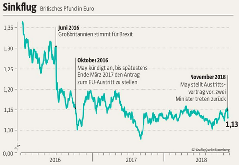
Source: Süddeutsche Zeitung am Wochenende, 17./18. November 2018, year 74, week 46, No. 265, p. 1 (front page).
1.2 International investments
Investing, whether through holding a currency or storing purchasing power, is inherently speculative, regardless of whether the investment is domestic or international. When you hold a foreign currency, it’s crucial to acknowledge that its value can both appreciate and depreciate. Currency values can fluctuate significantly over time due to factors such as economic policy, market sentiment, and global events. In the following sections, I will present a framework to help understand the key determinants of the rate of return on your investment. As illustrated in Figure 1.11, we will explore how a country’s interest rates, trade balances, price levels, and exchange rates are interconnected and must be analyzed together, rather than in isolation.
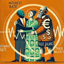
Source: Generated using OpenAI (2025).
1.2.1 Foreign exchange reserves
Currencies serve as a store of value, an important function in the financial world. Foreign exchange reserves are assets held on reserve by a central bank in foreign currencies, which can include bonds, treasury bills, and other government securities. The primary purpose of holding foreign exchange reserves is to manage the exchange rate of the national currency and ensure the stability of the country’s financial system.
Accordingly to the Currency Composition of Official Foreign Exchange Reserves (COVER) database of the International Moentary Fund (IMF), the total foreign exchange reserves in Q3 2023 had been 11,901,53 billion U.S. Dollar. That is, $ 11,901,530,000,000!
The size of a country’s foreign exchange reserves can be influenced by various factors, including its balance of trade, exchange rate policies, capital flows, and the overall health of its economy. While having substantial reserves is generally seen as a sign of economic strength and stability, excessively accumulating reserves can also indicate underlying economic imbalances or protectionist policies.
1.2.2 Three components of the rate of return
An investment usually has different characteristics such as the default risk, opportunities, and liquidity. These characteristics and individual preferences are important to decide which investment is superior. In this course, however, we mostly refrain from discussing sophisticated features of investments here. We focus on the most important feature of an investment, that is, the rate of return. In particular, three components are important to calculate the rate of return:
1.2.2.1 Interest rate
The interest rate of an investment is a crucial factor that determines the return earned on invested capital over a specific period. It represents the percentage of the initial investment that is paid back to the investor as interest or profit. Formally, we can write: \[ \underbrace{I_{t-1}}_{\text{investment in {t-1}}} \cdot\quad \underbrace{(1+i)}_{1+\text{interest rate}} = \underbrace{I_{t}}_{\text{payout amount in t}} \tag{1.1}\] where \(I\) denotes the value of an asset measured in € in the respective time period \(t\).
1.2.2.2 Exchange rate
When investing in assets denominated in foreign currencies, investors need to convert their domestic currency into the foreign currency at the prevailing exchange rate. After the investment has been paid out in the foreign country, the investor must convert the foreign currency back to his home currency. Thus, the initial cost of the investment and the subsequent returns are influenced by the exchange rate at the beginning and the end of the investment.
Formally, we can write if the an investment takes in foreign country, that is, Turkey between \(t-1\) and \(t\): \[ I^{\text{€}}_{t-1}\cdot E_{t-1}^{\frac{\text{₺}}{\text{€}}} \cdot E_{t}^{\frac{\text{€}}{\text{₺}}}= I_{t}^{\text{€}} \tag{1.2}\]
1.2.2.3 Inflation
Inflation refers to the quantitative measure of the rate at which prices, represented by a basket of goods and services, increase within an economy over a specific period. Conversely, negative inflation is termed deflation. Mathematically, inflation can be defined as follows:
\[ \pi = \frac{P_t - P_{t-1}}{P_{t-1}} = \frac{P_t}{P_{t-1}} - 1 \]
Where \(\pi\) represents the inflation rate and \(P_t\) denotes the price at time \(t\). When inflation affects all prices, it also impacts the value of assets in which investors are invested. This relationship can be expressed as:
\[ I_t = I_{t-1} \cdot (1+\pi) \tag{1.3}\]
1.2.3 Rate of return of an investment abroad
The rate of return, \(r\), is the growth rate of an investment over time and can be described as follows: \[\begin{align*} r=& \frac{I^{\text{€}}_t-I_{t-1}^{\text{€}}}{I_{t-1}^{\text{€}}}=\frac{I^{\text{€}}_t}{I^{\text{€}}_{t-1}}-1, \end{align*}\]
Combining Equation 1.1, Equation 1.2, and Equation 1.3, we can describe the value of our investment in period \(t\) as follows: \[ I_{t}^{\text{€}}= I_{t-1}^{\text{€}} \cdot (1+i^{*}) \cdot E_{t-1}^{\frac{\text{₺}}{\text{€}}} \cdot E_{t}^{\frac{\text{€}}{\text{₺}}} \cdot (1+\pi^{*}), \tag{1.4}\] where \(I_{t-1}^{\text{€}}\) denotes the initial investment, \(i^{*}\) denotes the interest rate abroad and \(\pi^{*}\) the inflation abroad. Dividing by \(I_{t-1}^{\text{€}}\) and subtracting \(1\) from both sides of Equation 1.4, we see that the rate of return for an investment abroad, \(r^{*}\), has three determining factors, that are: interest rate \((1+i^*)\), inflation \((1+\pi)\), and the change of exchange rates over time \((E_{t-1}^{\frac{\text{₺}}{\text{€}}} \cdot E_{t}^{\frac{\text{€}}{\text{₺}}})\): \[\begin{align*} \underbrace{\frac{I_{t}^{\text{€}}}{I_{t-1}^{\text{€}}}-1}_r^*&= (1+i^{*})\cdot (1+\pi^{*}) \cdot \underbrace{E_{t-1}^{\frac{\text{₺}}{\text{€}}} \cdot E_{t}^{\frac{\text{€}}{\text{₺}}}}_\alpha -1 \end{align*}\] \[ r^*= (1+i^{*})\cdot (1+\pi^{*}) \cdot \alpha -1 \tag{1.5}\] with
- \(\alpha=1\) if the exchange rate does not change over time and
- \(\alpha>1\) if the home currency € depreciates or
- \(\alpha<1\) if the home currency € appreciates.
So the exchange rate changes over time work as a third factor of your rate of return.
By assuming no inflation (\(\pi^{*}=0\)), we can write
\[
\begin{aligned}
r^*&=(1+i^{*}) \cdot \alpha -1\\
\Leftrightarrow r^*&=\alpha +\alpha i^{*} -1.
\end{aligned}
\tag{1.6}\] Reorganizing Equation 1.6 helps to interpret it. Firstly, let us expand the right hand side of this equation adding and subtracting \(i^*\) which obviously does not change the sum of the right hand side of the equation. Secondly, re-write the equation and thirdly, set \((\alpha-1)=w\): \[
\begin{aligned}
\Leftrightarrow r^*&=\alpha +\alpha i^{*}-1+i^*-i^*\\
\Leftrightarrow r^*&=\alpha-1+i^* +\alpha i^{*}-i^*\\
\Leftrightarrow r^*&=\underbrace{(\alpha -1)}_w+i^* +i^{*}\underbrace{(\alpha -1)}_w\\
\Leftrightarrow r^*&=w+i^* +i^{*}w
\end{aligned}
\tag{1.7}\]
This equation outlines the rate of return on an investment in a foreign country, influenced by two primary factors: \(i^*\) and \(w\).
Assuming that the product \(iw\) is very small, we can say that the rate of return equals approximately the interest rate plus the rate of depreciation: \[r^{*}=w+i^{*}.\] This approximation is often called the simple rule for \(r\).
1.2.4 The interest parity condition
Assume the rate of return is lower domestically than it is for investments abroad. Representing the foreign country with an asterisk \((*)\), this situation, where investing money abroad is more profitable, can be expressed as:
\[\begin{align*} r&<r^{*}. \end{align*}\] Given that domestically the rate of return, \(r\), equals the interest rate, \(i\), assuming zero inflation, and that the simple rule for an investment abroad is described by \(r^{*} = w + i^{*}\), we can rewrite the equation as: \[ i< w+i^{*}. \] What would happen if financial market actors became aware of this?
Market participants would likely convert their domestic currency into the foreign currency to invest abroad, increasing demand for the foreign currency. Consequently, the foreign currency would appreciate, becoming relatively more expensive. This implies that \(w\) is negative. This appreciation process halts when investing abroad no longer offers a higher return. If the attractiveness of investments is equalized, the FOREX is in equilibrium. The deposits of all currencies offer the same expected rate of return. In other words, in equilibrium the exchange rate, \(w\), assures that the rate of return from the home country, \(r\), is equal to the rate of return in any foreign country, denoted with an asterisk (\(*\)):
\[\begin{align} r&=r^{*}\\ i&= w + i^{*}\\ \end{align}\] \[ \Leftrightarrow w= i-i^{*} \tag{1.8}\]
The interest parity condition (Equation 1.8) enables us to analyze how variations in interest rates and expected exchange rates affect current exchange rates through comparative static analysis of the equation: \[ \frac{\partial w}{\partial i} > 0; \quad \frac{\partial w}{\partial i^*} < 0. \] This means:
- An increase in the domestic interest rate results in a positive change in the depreciation rate, leading to the depreciation of the domestic currency.
- An increase in the foreign interest rate causes a negative change in the depreciation rate, resulting in the appreciation of the domestic currency.
1.2.5 The theory in real markets: Unpegging the Swiss Franc
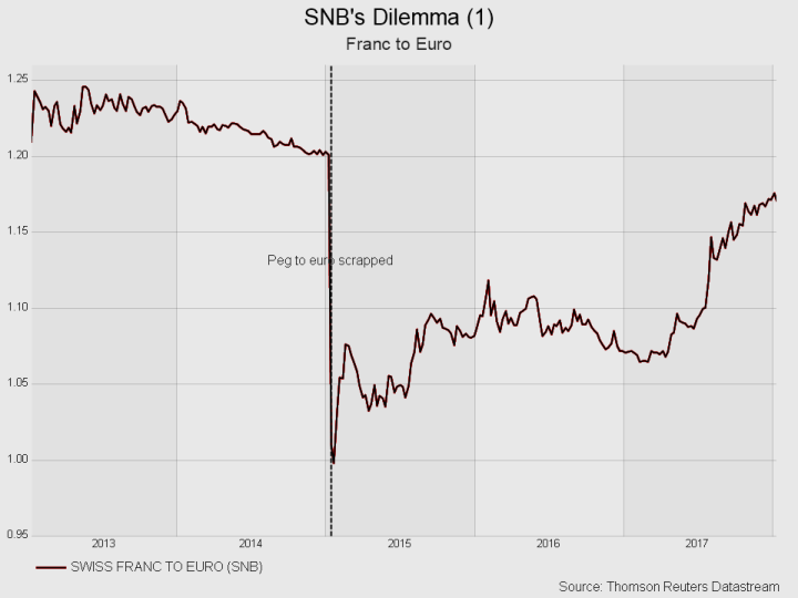
You might now question whether this theory of the interest parity condition truly holds in real-world markets. Analyzing international markets and the FOREX empirically is challenging due to the frequent occurrence of both large and small exogenous shocks on a global scale, each impacting market outcomes in various ways. Furthermore, market dynamics are often influenced by emotions and speculation rather than solely measurable facts. However, there are instances where the shocks are so significant that the fundamental forces driving the market become visible, even without a sophisticated empirical identification strategy that controls for confounding effects. The case study of the unexpected unpegging of the Swiss Franc serves as a poignant example. It vividly demonstrates that the principles underpinning the interest parity condition are not merely theoretical constructs but actively influence real market behaviors.
Until early 2015, the Swiss National Bank (SNB) had a policy goal to maintain the franc above the cap of 1.20 Francs per Euro, aiming to protect exporters and combat deflationary pressures. However, in a surprising move, the SNB unpegged the Franc in 2015. This decision was influenced by the appreciation pressure on the Franc, as many investors many investors wanted to store their assets in the Swiss Franc. Following the SNB’s announcement, the exchange rate plunged from 1.20 to 1.00 Franc per Euro \((E^{\frac{CHF}{\text{€}}})\), as illustrated in Figure 1.12 (a) Almost simultaneously, the interest rate experienced a decline, as depicted in Figure 1.12 (b). These developments align precisely with what the interest parity condition would predict, demonstrating its applicability in real-world financial market dynamics.
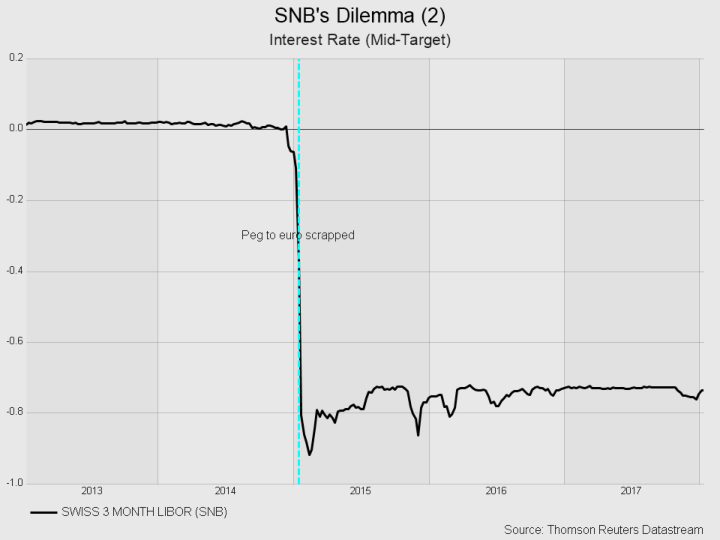
To analyze the relationship between changes in exchange rates and interest rates, we need to consider the interest parity assumption of Equation 1.8: \[ w= i-i^{*} \] where \[w=\frac{E_{t}^{\frac{\text{€}}{CHF}}}{E_{t-1}^{\frac{\text{€}}{CHF}}}-1.\] In January 2015, the exchange rate \(E^{\frac{CHF}{\text{€}}}\) decreased from 1.20 to 1.00. Alternatively, we can express this change in direct quotation, noting that the exchange rate \(E^{\frac{\text{€}}{CHF}}\) increased from \(E^{\frac{\text{€}}{CHF}}_{t-1}\approx \frac{1}{1.20}\approx 0.83\) to \(E^{\frac{\text{€}}{CHF}}_{t}\approx 1.00\), resulting in \[ w=\frac{E_{t}^{\frac{\text{€}}{CHF}}}{E_{t-1}^{\frac{\text{€}}{CHF}}}-1=\frac{1}{0.83}-1=0.20. \]
Since \(w > 0\), the fraction on the left-hand side of the interest rate parity equation must also be positive, as already mentioned. This implies that \[i - i^* > 0,\] which means that an interest rate spread must occur. This condition can occur if the foreign interest rate \(i^*\) decreases or the domestic interest rate \(i\) increases. In our observations, we can indeed see a pattern that is consistent with our theoretical expectations.
It is important to acknowledge that our theoretical framework simplifies the complex interplay of factors that influence both exchange rates and interest rates. Despite this simplification, the model highlights the key forces driving market dynamics. However, it is important to point out that the actual numbers may not perfectly match our theoretical predictions in quantitative terms, as shown in Figure Figure 1.13.
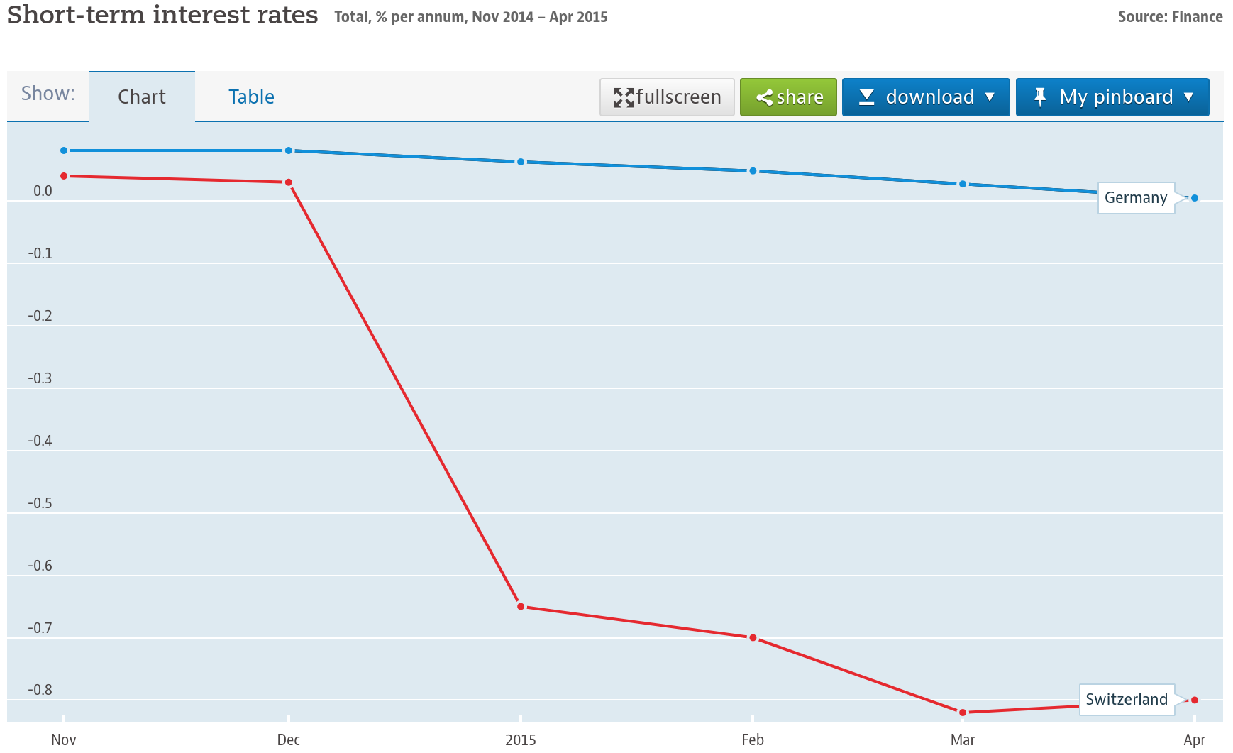
Source: Data are taken from the OECD and show the total, % per annum.
1.2.6 The Fisher Effect
The Fisher Effect is an economic theory proposed by economist Irving Fisher (1867-1947), which describes the relationship between (expected) inflation and both nominal and real interest rates.
According to the Fisher Effect, the nominal interest rate is equal to the sum of the real interest rate and the (expected) inflation rate. In formula terms, it is often expressed as: \[ r=i+\pi. \tag{1.9}\]
We can derive Equation 1.9 assuming that the exchange rate is stable over time \[ \left( E_{t-1}^{\frac{\text{€}}{\text{₺}}} =E_{t}^{\frac{\text{€}}{\text{₺}}} \Leftrightarrow \frac{E_{t-1}^{\frac{\text{€}}{\text{₺}}}}{E_{t}^{\frac{\text{€}}{\text{₺}}}}=1 \Leftrightarrow \alpha=1 \right) \] and using this in Equation 1.5, we get: \[\begin{align} r^*&= (1+i^{*})\cdot (1+\pi^{*}) \cdot \underbrace{\alpha}_{=1} -1 \\ \Leftrightarrow r=& i+ \pi+ \pi i \end{align}\] Assuming that the product \(\pi i\) is very small, we can say that the rate of return equals approximately the interest rate plus the inflation rate. This approximation shown in Equation 1.9 is often called the Fisher Effect.
Considering now cross-country differences in their rate of return, we can explain the rate of return spread by the inflation rate and the nominal interest rate spread as follows: \[r_{GER}-r_{TUR}= \pi_{GER}-\pi_{TUR} + i_{GER}-i_{TUR}. \tag{1.10}\]
We have learned in Section 1.2.4 (the interest parity condition) that the rate of return can differ only in the short run and will be equal across countries in the long run (\(r_{GER} - r_{TUR} = 0\)). Utilizing this concept in Equation 1.9, we can demonstrate that the nominal interest rates of countries will adjust to accommodate any changes in (expected) inflation, and vice versa:
\[i_{GER} - i_{TUR} = \pi_{GER} - \pi_{TUR}.\]
1.3 Balance of payments
1.3.1 Introduction
The Balance of Payments is a record of a country’s financial transactions with the rest of the world. It tracks the money flowing in and out through various economic activities. If we account for all transactions, the inflow and outflow should theoretically balance. Before I elaborate on this concept, let’s clarify some key terms:
- Exports: Goods and services sold to other countries.
- Imports: Goods and services bought from other countries.
- Trade balance: The difference between the value of goods and services a country sells abroad and those it buys from abroad, also known as net exports.
- Trade surplus: When a country sells more than it buys, resulting in a positive trade balance.
- Trade deficit: When a country buys more than it sells, leading to a negative trade balance.
- Balanced trade: When the value of exports equals imports.
- Net capital outflow: The difference between the purchase of foreign assets by domestic residents and the purchase of domestic assets by foreigners. This equals net exports, indicating that a country’s savings can fund investments domestically or abroad. We will elaborate on that later on in greater detail.
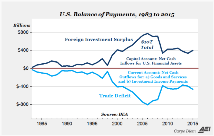
Exercise 1.12 Figure 1.14 represents the foreign investment surplus and the trade deficit. Discuss why the two lines mirror each other. Could this be a coincidence?
1.3.2 The payments must be balanced!
Every international financial transaction is essentially an exchange. When a country sells goods or services, the buying country compensates by transferring assets. Consequently, the total value of goods and services a country sells (its net exports) must be equal to the value of assets it acquires (its net capital outflow).
The Balance of Payments account consists of two primary components:
The Current account (Leistungsbilanz) measures a country’s trade balance (goods and services exports minus imports) plus the effects of net income and direct payments. It is positive, if a country is a net lender to the rest of the world and negative, if it is a net borrower from the rest of the world. In other words, an account surplus increases a country’s net foreign assets.
The Capital account (Kapitalbilanz) reflects the net change in ownership of national assets. Capital can flow in the form of following:
- Foreign Direct Investment (FDI): It involves investing in foreign companies with the intention of controlling or significantly influencing their operations.
- Foreign Portfolio Investment (FPI): This type of investment is in foreign financial assets, such as stocks and bonds, where the investor does not seek control over the companies.
- Other investments: This includes capital flows into bank accounts or funds provided as loans. It also encompasses the reserve account, which is managed by the central bank responsible for buying and selling foreign currencies.
Ignoring statistical effects, these two subaccounts must sum to zero.
While it’s true that the overall totals of payments and receipts must inherently balance, certain transaction types can create imbalances, leading to either deficits or surpluses. These imbalances may manifest in various sectors such as trade in goods (commodities), services trade, foreign investment income, unilateral transfers (including foreign aid), private investment, and the flow of gold and currency between central banks and treasuries, among other international dealings. It’s crucial to note, though, that the accounting framework ensures these surpluses and deficits ultimately zero out, adhering to the principles of double-entry bookkeeping.
| Receipt (credit) | Payments (debits) | ||
|---|---|---|---|
| Current Account | |||
| 1. Export of goods and services | 800 | 3. Import of goods and services | 600 |
| 2. Unilateral receipts | 300 | 4. Unilateral payments | 390 |
| Total | 1100 | Total | 990 |
| Capital Account | |||
| 5. Borrowings | 700 | 7. Lendings | 750 |
| 6. Sale of gold/assets | 100 | 8. Purchase of gold/assets | 150 |
| Total | 800 | Total | 900 |
| Errors and omissions | 10 | ||
| Total | 1900 | Total | 1900 |
1.3.3 A normative discussion of imbalances in the capital and current account
Normatively discussing imbalances in the capital and current accounts of countries involves evaluating these phenomena from a perspective of what ought to be, considering ethical, practical, and policy implications. These imbalances are not merely numerical figures; they reflect underlying economic activities and policy decisions with significant implications for national and global economic health.
1.3.3.1 Current account imbalances
The current account includes trade in goods and services. A surplus in the current account indicates that a country is exporting more goods than it imports.
Surpluses: Normatively, persistent current account surpluses might be viewed as a sign of a country’s competitive strength in the global market. However, they can also indicate underconsumption or insufficient domestic investment, suggesting that a country is not fully utilizing its economic resources to improve the living standards of its population. Furthermore, large surpluses can lead to tensions with trading partners and might prompt accusations of unfair trade practices or currency manipulation.
Deficits: On the other hand, persistent deficits could signal domestic economic vitality and an attractive environment for investment, reflecting high consumer demand and robust growth. Yet, they can also indicate structural problems, such as a lack of competitiveness, reliance on foreign borrowing to sustain consumption, or inadequate savings rates. Over time, large deficits may lead to unsustainable debt levels, making the country vulnerable to financial crises.
1.3.3.2 Capital account imbalances
The capital account records the net change in ownership of national assets. It includes the flow of capital into and out of a country, such as investments in real estate, stocks, bonds, and government debt.
Inflows: Capital account inflows can signify strong investor confidence in a country’s economic prospects, potentially leading to increased investment and growth. However, excessive short-term speculative inflows can destabilize the economy, leading to asset bubbles and subsequent financial crises when the capital is suddenly withdrawn.
Outflows: Capital outflows might indicate a lack of confidence in the domestic economy or better opportunities abroad. While some level of outflow is normal for diversified investment portfolios, large and rapid outflows can precipitate a financial crisis by depleting foreign reserves and putting downward pressure on the currency.
1.3.4 A formal representation
In the following, I present a streamlined perspective on the global trading system. This overview does not engage with the benefits or drawbacks of maintaining trade surpluses or deficits, a subject that warrants its own discussion. However, it aims to identify the factors influencing current account deficits and surpluses.
1.3.4.1 Closed economy
Within a closed economy, we identify three principal actors: households, firms, and the government. Let’s define \(C\) as the consumption of goods and services by households, encompassing necessities and luxuries like food, housing, and entertainment. Let \(G\) represent government expenditures, which cover infrastructure, social services, military outlays, education, and more. Lastly, \(I\) symbolizes the investment by firms in assets such as machinery, buildings, and research and development. Given these components, the total economic output, \(Y\), can be expressed by the fundamental equation of economics as:
\[ Y = C + I + G. \]
This equation encapsulates the aggregate spending within a closed economy, highlighting the interplay between consumption, investment, and government expenditure in determining overall economic activity.
If we define national savings, \(S\), as the share of output not spent on household consumption or government purchases, then the investments, \(I\), must be equal to the savings in a closed economy: \[\begin{align*} Y &= C + I + G\\ \Leftrightarrow \underbrace{Y - C - G}_S &= I \\ \Leftrightarrow S &= I, \end{align*}\]
This implies that within a closed economy, any portion of the output that is not consumed—either privately by households (\(C\)) or by the government (\(G\))—necessarily must be allocated towards investment (\(I\)). Thus, the equation underscores a foundational economic principle: the total output of an economy (\(Y\)) is either consumed or invested, leaving no surplus output.
1.3.4.2 Open economy
In an open economy, the dynamics of household consumption, government expenditures, and firm investments extend beyond domestic production to include imports from and exports to foreign markets. Thus, an economy can import and export goods. Denoting imports by \(IM\) and exports by \(EX\), we can re-write the fundamental equation of economics by adding the concept of net exports (\(NEX\)), the difference between a country’s exports and imports. A positive net export value (\(EX > IM\)) indicates a trade surplus, reflecting that the economy exports more than it imports. Conversely, a negative net export value (\(EX < IM\)) signifies a trade deficit, where imports exceed exports:
\[\begin{align*} Y &= C + I + G + \underbrace{EX - IM}_{NEX}\\ \Leftrightarrow \underbrace{Y - C - G}_S &= I + NEX\\ \Leftrightarrow \underbrace{S-I}_{NCO} &= NEX \end{align*}\]
In scenarios where investment equals savings (\(I = S\)), the economy’s net exports are zero, reflecting a balance between domestic production not allocated towards household or government consumption and investments. However, when an economy experiences a trade surplus (\(NEX > 0\)), such as Germany in recent decades, it implies that domestic savings exceed investments. This surplus indicates that the country produces more than it spends on domestic goods and services, channeling excess savings into investments abroad. Thus, savings not utilized domestically (\(S - I\)) are equivalent to the net capital outflow (\(NCO\)), establishing a direct link between a country’s trade surplus and its role as a global lender or investor:
\[ NCO = NEX \]
Net exports must be equal to net capital outflow
The accounting identities above simply state that there is a balance of payments. The Balance of Payment accounts are based on double-entry bookkeeping and hence the annual account has to be balanced. If an economy has a current account trade deficit (surplus), it is offset one-to-one by a capital account surplus (deficit) to assure a balance of payments. In other words, if an economy wants to import more goods than it produces, it must attract foreign capital to be invested at home.
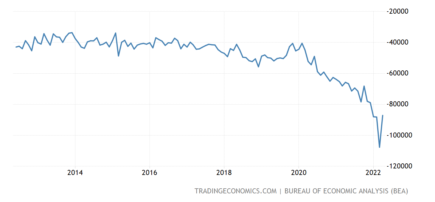
1.3.5 Case study: U.S. trade deficit
Consider a scenario where the United States is unable to attract sufficient capital flows from abroad to finance its trade deficit. In such a case, American consumers continue purchasing foreign goods with US Dollars, leading to an outflow of US Dollars that surpasses inflow. This imbalance results in an increased supply of US Dollars relative to its demand, causing the value of the US Dollar to depreciate. A depreciated US Dollar would, in theory, make US exports more competitive (cheaper for foreign buyers) and imports more costly, thereby potentially reducing the current account deficit. However, the trade deficit of the United States has remained relatively stable, and the US Dollar has not experienced significant depreciation. This stability is partly why former President Trump criticized other countries for allegedly manipulating their currencies, see Figure 1.15.
Trump’s stance on the trade deficit was clear: he perceived it as detrimental to the United States. He advocated for a weaker dollar and lower interest rates to address this issue. A weaker dollar would render American products more affordable internationally, stimulating exports and discouraging imports. Concurrently, lower interest rates in the United States would diminish the country’s appeal for foreign capital investments (\(I\) would decrease), leading to reduced net capital inflows. This adjustment would, in turn, decrease the Capital Account surplus and, by extension, shrink the Current Account deficit. Specifically, Trump accused the Chinese government and the European Central Bank of implementing policies that undervalue their currencies (the Renminbi and the Euro), thereby gaining an unfair advantage in trade.
As Trump thinks a trade deficit is bad for the United States, he would like to have a weak dollar and low interest rates. A weak dollar makes American products cheap for the rest of the world and has positive effects on exports and negative on imports. A low interest rate in the United States would make the country less attractive for foreign capital investments (\(I\) would become smaller), meaning the net capital inflows would decrease and so would the Capital Account’s surplus (and with it, the Current Account deficit would become smaller). In concrete terms, he claims that in particular the Chinese government and the European Central Bank run policies that keep their currencies (Renminbi and Euro) cheap.
Despite significant efforts by President Trump to reduce the U.S. trade deficit, the endeavor did not achieve its intended outcome, as illustrated in Figure 1.16. One likely reason for this shortfall was the reduction of taxes for large corporations, which enhanced the rate of return on investments. This policy made investing in the U.S. more appealing to foreign investors, potentially counteracting efforts to diminish the trade deficit.