6 Appendix

6.1 Microeconomic preliminaries

In this appendix, I will cover several microeconomic preliminaries that are crucial for your understanding. These include:

1. Production Possibility Frontier (PPF): I will explain how the PPF curve graphically visualizes the production and growth of firms and countries.
2. Indifference curves: I will discuss how indifference curves represent different bundles of goods at which consumers are indifferent.
3. Budget constraints: I will show you how to graphically sketch budget constraints, which play a significant role in consumer decision-making.
4. Consumption choices: I will explore how the concepts of PPF, indifference curves, and budget constraints come together to explain consumer consumption choices.
5. Competitive market prices: I will explain how prices on competitive markets are determined through the interaction of producers and consumers.

6.1.1 Production possibility frontier curve

The production possibility frontier curve

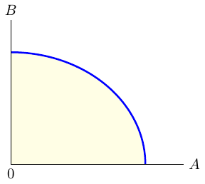
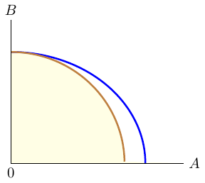
The production possibility frontier curve (PPF) as shown in figure 6.1 provides a graphical representation of all possible output options for two products when all available resources and factors of production are fully and efficiently utilized within a given time frame. The PPF serves as the boundary between combinations of goods and services that can be produced and those that cannot.

The PPF is an invaluable tool for illustrating the implications of scarcity, as it offers insights into production efficiency, opportunity costs, and tradeoffs between different choices. Typically, the PPF exhibits concavity since not all factors of production can be used equally productive in all activities.

Economic growth refers to the sustained expansion of production possibilities. An economy experiences growth through advancements in technology, enhancements in labor quality, or increases in capital quantity. As an economy`s resources increase, its production possibilities expand, causing the PPF to shift outward. It is worth noting that you can use the PPF to explain production in an “economy” or in a “firm”, respectively.

Production efficiency arises when it is impossible to produce more of one good or service without producing less of another. When production occurs directly on the PPF, it signifies efficiency. On the other hand, if production takes place inside the PPF, there is potential to produce more goods without sacrificing any existing ones, indicating inefficiency. When production lies on the PPF, a tradeoff emerges because obtaining more of one good necessitates giving up some quantity of another. This tradeoff incurs a cost, known as an opportunity cost.

Exercise 6.1 Understanding production

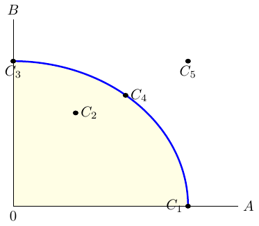
1. Figure 6.2 shows a PPF and five conceivable production points, \(C_i\), where \(i\in \{1,\dots,5\}\). Explain the figure using the following terms: attainable point; available resources, unattainable, inefficient, efficient point.

Production and different consumptions points

2. What would happen to the PPF if the technology available in a country and needed for the production process became better?

3. What would happen to the PPF if the resources available in a country and needed in the production process of both goods shrank?

4. What would happen to the PPF if the resources (technology) available in a country that are needed in the production process\(\dots\)

   1. \(\dots\) for both goods increased (improved)?
   2. \(\dots\) for good A shrank (got worse)?
   3. \(\dots\) for good B increased (improved)?

5. Does the shape of the PPF tell us anything about economies of scale in the production process?

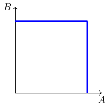
6. Figure 6.3 shows an extreme PPF. How can such a PPF be explained?

Extreme production possibility frontier curve

Please find solution to the exercise in the appendix.

6.1.2 Indifference curves and Isoquants

Indifference curve

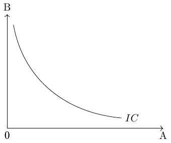
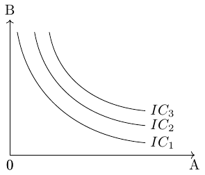
Combinations of two goods that yield the same level of utility for consumers are represented by indifference curves, see figure 6.4. These curves illustrate the various bundles of goods where consumers are equally satisfied. That means all points on an indifference curve represent the same level of utility. The shape of the indifference curve is determined by the underlying utility function, which captures the preferences of consumers for consuming different combinations of the two goods.

The slope of an indifference curve indicates the rate at which the two goods can be substituted while maintaining the same level of utility for the consumer. Technically, the slope represents the marginal rate of substitution, which is equal to the absolute value of the slope. It measures the maximum quantity of one good that a consumer is willing to give up in order to obtain an additional unit of the other good.

It is assumed that consumers aim to attain the highest possible indifference curve because a higher curve, located further to the right on a coordinate system, represents a higher level of utility. In figure 6.5 for example, \(IC_1\) represents a lower level of utility than \(IC_2\).

Indifference curve

Similar to the concept of indifference curves, an isoquant shows the combinations of factors of production that result in the same quantity of output.

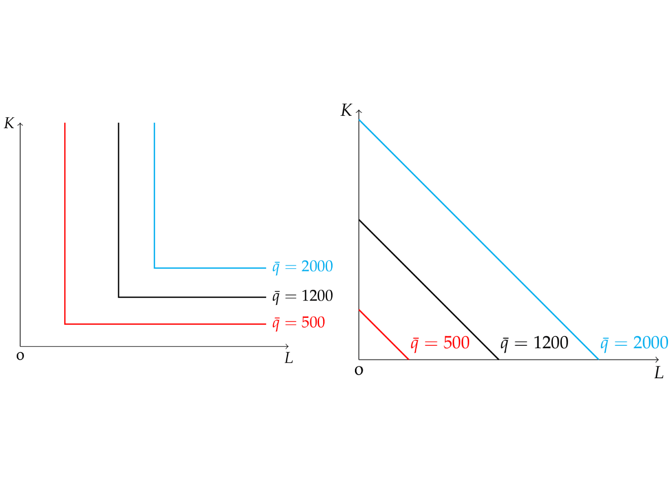
Figure 6.6: Perfect complements or substitutes

Exercise 6.2 Isoquants

1. Which of the two plots of figure 6.6 show isoquants when factors of production are perfect complements and perfect substitutes, respectively?

2. Discuss the features of a Cobb-Douglas PF with respect to returns to scale and marginal product of production for both inputs. Sketch the total output curve in an output-\(K\) and an output-\(L\) quadrant. Sketch the isoquants for different levels of production.

Please find solution to the exercise in the appendix.

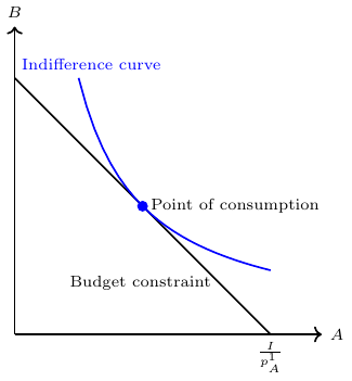
6.1.3 Budget constraint

In microeconomics, the concept of a budget constraint plays a vital role in understanding consumer decision-making and helps to analyze consumer choices and trade-offs. The budget constraint represents the limitations faced by consumers in allocating their limited income across different goods and services. The budget constraint indicates that the total expenditure on goods and services, calculated by multiplying the prices of each item by its corresponding quantity, must be less than or equal to the consumer’s income. Mathematically, the budget constraint can be expressed as: \[ P_1 \cdot Q_1 + P_2 \cdot Q_2 + \ldots + P_n \cdot Q_n \leq I \] where \(P_n\) represent the prices of goods, \(Q_n\) denote the quantities of goods \(n\) consumed. \(I\) denotes the consumer’s income or their budget.

Consumers strive to maximize their utility by selecting the optimal combination of goods and services within the constraints imposed by their limited income. This involves making decisions about how much of each good to consume while staying within the budgetary limits. The graphical representation of the ideal consumption point is depicted in Figure 6.7.

By studying the budget constraint, economists can gain insights into consumer behavior, price changes, and the impact of income fluctuations on consumption patterns.

Indifference curve

6.2 Logarithmic and exponential function

Logarithmic and exponential function

Logarithmic and exponential function zoomed in

6.2.1 Logarithmic function

Maybe you have heard about the logarithm, and I’m quite sure you know the ‘log’ button on your calculator. If you wonder what it actually is and why it is so important for calculating with growth rates, this section is for you.

Consider the following equations and then explain to me what the logarithm is:

\[\begin{align*} 2\cdot2\cdot2\cdot2 &= 16 \\ 2^4 &= 16 \\ 2 &= 16^{\frac{1}{4}} \\ \log_2 16 &= 4 \end{align*}\]

Now, let us abstract from that concrete example and generalize things a bit:

\[\begin{align*} x^n &= y \\ \log_x y &= n \\ \log x^n &= \log y \\ n\cdot \log x &= \log y \\ n &= \frac{\log y}{\log x} \end{align*}\]

Here are some more examples:

\[\begin{align*} 4 &= \frac{\log 16}{\log 2} \\ \log_{10}16 &= 1.20411998265592 \\ \log_{10}2 &= 0.301029995663981 \\ \log 16 &= 1.20411998265592 \\ \log 2 &= 0.301029995663981 \\ \end{align*}\]

Exercise 6.3 Calculate with log

Calculate a logarithmic function without a calculator. Hint: The result is an integer.

• \(\log_2 16 = ?\)
• \(\log_3 243 = ?\)
• \(\log_5 125 = ?\)
• \(\log_3 81 = ?\)
• \(\log_2 \left(\frac{1}{8}\right)\)

Please find solution to the exercise in the appendix.

---

6.2.2 Exponential function

6.2.2.1 Definition

Let us consider the function \(f(x) = 2^{x}\) in table Table 1 and figure 6.10.

Table 1: The exponential function \(2^{x}\) in a table

\(x\)	\(f(x)\)	\((x,f(x))\)
\(-3\)	\(2^{-3} = \frac{1}{8}\)	\((-3, \frac{1}{8})\)
\(-2\)	\(2^{-2} = \frac{1}{4}\)	\((-2, \frac{1}{4})\)
\(-1\)	\(2^{-1} = \frac{1}{2}\)	\((-1, \frac{1}{2})\)
\(0\)	\(2^{0} = 1\)	\((0 ,1)\)
\(1\)	\(2^{1} = 2\)	\((1, 2)\)
\(2\)	\(2^{2} = 4\)	\((2,4)\)
\(3\)	\(2^{3} = 8\)	\((3, 8)\)

The exponential function \(2^{x}\) visualized

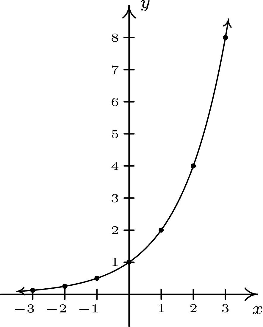
A function of the form \(f(x) = b^{x}\) where \(b\) is a fixed real number, \(b > 0\), \(b \neq 1\) is called a base \(b\) exponential function.

• Therefore, \(b\) is the factor by which \(f(x)\) increases or decreases when \(x\) increases by one unit.
• For \(b > 1\), the function \(f(x)\) is strictly increasing.
• For \(0 < b < 1\), the function \(f(x)\) is strictly decreasing.

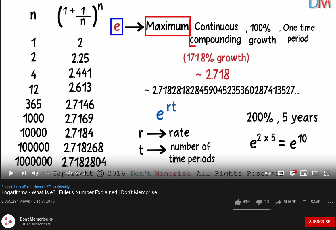
6.2.2.2 The number \(e\)

The most important base for exponential functions is the irrational number

\(e \approx 2.71828182845904523536028747135266249775724709369995\)

It is sometimes called Euler’s number, after the Swiss mathematician Leonhard Euler (1707-1783). It can be expressed as:

• \(e = \sum \limits _{n=0}^{\infty }{\frac {1}{n!}} = 1+{\frac {1}{1}}+{\frac {1}{1\cdot 2}}+{\frac {1}{1\cdot 2\cdot 3}}+\cdots\)

• \(e^{x} = 1+{x \over 1!}+{x^{2} \over 2!}+{x^{3} \over 3!}+\cdots = \sum _{n=0}^{\infty }{\frac {x^{n}}{n!}}\)

• \(e^k = \lim _{n\to \infty }\left(1+{\frac {k}{n}}\right)^{n}\)

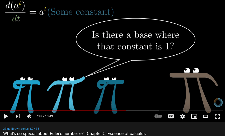
Watch the YouTube clips Logarithms - What is e? | Euler’s Number Explained | Don’t Memorise by Infinity Learn Class 9&10 (see figure 6.11) and What’s so special about Euler’s number e? | Chapter 5, Essence of calculus by 3Blue1Brown (see figure 6.12).

Euler’s number explained

What’s so special about Euler’s number e?

6.3 Solutions to exercises

Solution to exercise 2.3: What is the house of Santa Claus?

Forty-four ways to solve the puzzle²¹

Ten ways to fail in the puzzle²²

There are 44 solutions and only 10 different ways to fail. Thus, the probability to fail is about 18.5% and hence the probability to succeed is about 81.5%. In the course 10 persons participated in the poll. Here are the answers:

PINGO

Nobody came close to the correct probability.

Solution to exercise 2.6: Optimal vs. satisfactory solution

1. Collecting and analyzing the available information about a product is costly. It is also difficult to analyze the importance of product features for the intended purpose.
2. Individuals often use rules of thumb to make a satisfactory decision.
3. It is difficult to understand complex situations such as the market for financial products. For some people, it is simply not possible to find the best product in these complex markets.
4. Consumers are often confronted with many variants of a product. The differences are negligible and therefore it is not worthwhile for consumers to analyze the situation in detail. Thus, they make a decision that may not be optimal, but they are satisfied with it.

Solution to exercise 2.8: Lisa is pregnant

At the beginning of the Inferential Statistics course at summer 2020, I also asked student this question. Here are the results of the 16 students who participated:

Option	Frequency of answers	Percentage
a)	3	19%
b)	2	13%
c)	2	13%
d)	3	19%
e)	6	38%

How did they reach their answers? Like most people, they decided that Lisa has a substantial chance of having a baby with Down syndrome. The test gets it right 86 percent of the time, right? That sounds rather reliable, doesn’t it? Well it does, but we should not rely on our feelings here and better do the math because the correct result would be that there is just a 1.7 percent chance of the baby having a Down syndrome.

Now, let us proof the result that there is just a 1.7 percent chance of the baby having a Down syndrome using Bayesian Arithmetic which is explained in the following videos:

Also, consider this interactive tool here: https://www.skobelevs.ie/BayesTheorem/

Let \(A\) be the event of the Baby has a Down syndrom and \(B\) the test is positive. Then, \[\begin{align*} P(A)&=0.001\\ P(B\mid A)&=0.86\\ P(B\mid \neg A)&=0.05\\ P(B)&=\frac{999\cdot 0.05}{1000}+\frac{1\cdot 0.86}{1000}=\frac{50.81}{1000}=0.05081\\ P(A\mid B)&={\frac {P(B\mid A)P(A)}{P(B)}}=\frac{0.86 \cdot 0.001}{0.05081}=0.016925802 \end{align*}\]

Solution to exercise 3.1: Körth: example

\(\overline{O}_1=5; \overline{O}_2=1; \overline{O}_3=7; \overline{O}_4=3; \overline{O}_5=4\)

\(O_{ij}\)	\(k_1\)	\(k_2\)	\(k_3\)	\(k_4\)	\(k_5\)	\(\Phi(a_i)\)
\(a_1\)	3/5	0	1	1/3	1	0
\(a_2\)	4/5	0	4/7	2/3	1/4	0
\(a_3\)	4/5	-1	3/7	2/3	1/4	-1
\(a_4\)	1	1	3/7	1	1/4	1/4

\(a_4\succ a_1 \sim a_2 \succ a_3\)

Solution to exercise 3.7: Optimal vs. satisfactory solution

The example that is shown in Figure 7 of Finne (1998, p. 401) contains some errors. Here is the correct table including the Hurwicz-values (we assume \(\alpha=.5\)):

\(O_{ij}\)	\(min(\theta_1)\)	\(max(\theta_2)\)	\(H_i\)
\(a_1\)	36	110	73
\(a_2\)	40	100	70
\(a_3\)	58	74	66
\(a_4\)	61	66	63.5

Thus, the order of preference is \(a_4\succ a_3 \succ a_1 \succ a_2\).

Solution to exercise 3.2: Burgers and drinks

In figure 6.16, I marked all 19 possible bundles of burger and drinks of consumption. The budget constraint is shown by the solid line.

Possible consumption choices

• We now should calculate the utility of all 19 points, but only the red dots denote choices that may yield an optimal utility. The best utility is achieved when we buy 2 burgers and 3 drinks:

\[U=2^{0.6}3^{0.4}=2.35\]

• Solve:

\[ \mathcal{L}=B^{0.6}D^{0.4}+\lambda(3B+2D-12) \]

FOC: \[\begin{align*} 3B+2D-12&=0\\ 0.6B^{-0.4}D^{0.4}+3\lambda&=0\\ 0.4B^{0.6}D^{-0.6}+2\lambda&=0 \end{align*}\]

Solving the second and third FOC for \(\lambda\) and substituting \(\lambda\) gives:

\[B=D\]

which we can plug into the first FOC to obtain:

\[B^*=2.4 \quad \text{and} \quad D^*=2.4\]

Solution to exercise 3.4: Consumption choice

\[\begin{align*} \mathcal{L}&=A^{0.8}B^{0.2}+\lambda(6A+4B-30)\\ FOC: \frac{\partial \mathcal{L}}{\partial \lambda}&=6A+4B-30=0 \qquad (*)\\ \frac{\partial \mathcal{L}}{\partial A}&=0.8A^{-0.2}B^{0.2}+6\lambda=0 \qquad (**)\\ \frac{\partial \mathcal{L}}{\partial B}&=0.2A^{0.8}B^{-0.8}+4\lambda=0 \qquad (***) \end{align*}\] System of 3 equation with 3 unknowns can be solved in various ways. The easiest way is to solve () and (*) for \(\lambda\) and substitute it out:

• solve for \(\lambda\) \[\begin{align*} -\frac{2}{15} A^{-0.2}B^{0.2}&=\lambda \qquad (**')\\ -\frac{1}{20} A^{0.8}B^{-0.8}&=\lambda \qquad (***')\\ \end{align*}\]
• set both equations equal by substituting \(\lambda\) and solve for \(B\) \[\begin{align*} \frac{2}{15} A^{-0.2}B^{0.2}&= \frac{1}{20} A^{0.8}B^{-0.8}\\ B&=0.375A \qquad (****) %\\ \end{align*}\]
• Now, plug in \((****)\) into \((*)\) to get a number for \(A\) \[\begin{align*} 30&=6A+4\cdot 0.375 A\\ \Leftrightarrow 30&=7.5A\\ \Leftrightarrow A&=4 \end{align*}\]
• Use \(A=4\) in \((*)\) to get a number for \(B\) \[\begin{align*} 30&=6\cdot 4+4 B\\ \Leftrightarrow 6&=4B\\ B&=\frac{6}{4}=1.5 \end{align*}\]

Thus, we’d consume 4 units of good A and 1.5 of good B.

Solution to exercise 3.6: Cost-minimizing combination of factors

\[ \mathcal{L}=r_1+4r_2+\lambda\left(\frac{5}{4}r_1^{\frac{1}{2}}r_2^{\frac{1}{2}}-20\right) \] Taking the FOC we get \[r_1=4r_2\] using that in the constraint, we get \(r_1=32\) and \(r_2=8\).

Also see which uses this tool:

Solution to exercise 3.6: Lagrange with n-constraints

\[ \mathcal{L}(x_1, \dots, x_m, \lambda_i, \dots, \lambda_n)=f(\mathbf{x})+\lambda_1 g_1(\mathbf{x})+\lambda_2 g_2(\mathbf{x})+\ldots+\lambda_n g_n(\mathbf{x}) \] The points of local minimum would be the solution of the following equations: \[\begin{align*} \frac{\partial \mathcal{L}}{\partial x_{j}} &=0 \quad \forall j=1 \dots m \\ g_i(\mathbf{x}) &=0 \quad \forall i=1\dots n \end{align*}\]

Solution to exercise 3.9: To be vaccinated or not to be

1. \[\begin{align*} P(D)&=P(V)\cdot P(D|V)+(P(\neg V)\cdot P(D|\neg V))\\ &= .96\cdot .05 + .04 \cdot .09\\ &= 0.048 + 0.036 \\&= 0.084 \end{align*}\]
2. \[\begin{align*} P(V \mid D)={\frac {P(D\mid V)P(V)}{P(D)}}= \frac{.05\cdot .96}{.084}\approx .5714285 \end{align*}\]

Solution to exercise 3.10: To die or not to die

1. \[P(D) = 0.9\cdot0.2+0.1\cdot0.4=0.22\]
2. \[P(V\mid D)=\frac P(D\mid V)P(V)P(D)=\frac0.2\cdot 0.90.22=\frac0.0360.22\approx0.8181\] % \[P(\neg V\mid D)=\frac P(D\mid \neg V)P(\neg V)P(D)=\frac0.4\cdot 0.40.028=\frac0.020.028\approx0.71428\]
3. …

Solution to exercise 3.11: Corona false positive

In order to come to an answer, lets draw a table of the probabilities that may be of interest:

	A	\(\neg A\)	\(\sum\)
B	\(P(A\cap B)\)	\(P(\neg A \cap B)\)	\(P(B)\)
\(\neg B\)	\(P(A \cap \neg B)\)	\(P(\neg A \cap \neg B)\)	\(P(\neg B)\)
:—	:—:	:—:	:—:
	\(P(A)\)	\(P(\neg A)\)	1

Please note, the symbol $\neg$'' simply abbreviates’’ and the symbol $\cap$'' stands for’’. The probability of you having both the disease and a positive test, \(P(A \cap B)\), is easy to calculate: \[\underbrace{P(A \cap B)= P(B|A)P(A)}_{\text{a.k.a. multiplication rule}}=.99\cdot .001=.00099\] Also, it is straight forward to calculate the probability of having both, no infection and a positive test: \[ P(\neg A \cap B)= P(B|\neg A)P(\neg A)=.02\cdot .999 = .01998 \] Knowing that, it is clear that the overall probability of being diagnosed with Corona is \[P(B)=.00099+.0199=.02097\] That means, out of 1000 people about 21 are on average diagnosed with Corona while only one person actually is infected with Corona. Thus, your probability of having Corona once your test came out to be positive, \(P(A|B)\), is approximately \[P(A|B) \approx \frac{1}{21}=0,047619048\]

and more precisely \[ P(A|B)=\frac{P(A\cap B)}{P(B)}=\frac{.00099}{.02097}=0,0472103. \]

In other words, with a probability of more than 95%, you may go into quarantine without infection: \[ P(\neg A|B)=\frac{P(\neg A\cap B)}{P(B)}=\frac{.01998}{.02097}=0,9527897\quad (=1-P(A|B)) \] Given the accuracy of the test, this number appears to be rather high to many people. The high test accuracy of 99% and the rather low number of 2% false positives, however, is misleading. This is sometimes called the . The source of the fact that many people think \(P(A|B)\) is much lower is that they don’t consider the impact of the low probability of having the disease, \(P(A)\), on \(P(A|B)\), \(P(B|A)\), and \(P(B|\neg A)\) respectively (also, see the ). Moreover, many people don’t understand the false positive rate correctly.

To summarize, we know

	A	¬A	\(\sum\)
B	.00099	.01998	.02097
¬B	P(A ¬B)	P(¬A ¬B)	P(¬B)
—	.001	P(¬A)	1

The four remaining unknowns can be calculated by subtracting in the columns and adding across the crows, so that the final table is:

	A	¬A	\(\sum\)
B	.00099	.01998	.02097
¬B	.00001	.97902	.97903
—	.001	.999	1

Solution to exercise 3.12: Twelve cognitive biases

1. Ease of Recall: Individuals tend to consider events that are more easily remembered to be more frequent, regardless of their actual frequency.

2. Retrievability: Individuals’ assessments of event frequency are influenced by how easily information can be retrieved from memory.

3. Insensitivity to Base Rates: Individuals tend to ignore the frequency of events in the general population and focus instead on specific characteristics of the events.

4. Insensitivity to Sample Size: Individuals often fail to take sample size into account when assessing the reliability of sample information.

5. Misconceptions of Chance: Individuals expect random processes to produce results that look “random” even when the sample size is too small for statistical validity.

6. Regression to the Mean: Individuals fail to recognize that extreme events tend to regress to the mean over time.

7. Conjunction Fallacy: Individuals often judge that the occurrence of two events together is more likely than the occurrence of either event alone.

8. Confirmation Trap: Individuals tend to seek out information that confirms their existing beliefs and ignore information that contradicts them.

9. Anchoring: Individuals often make estimates based on initial values, and fail to make sufficient adjustments from those values.

10. Conjunctive- and Disjunctive-Events Bias: Individuals tend to overestimate the likelihood of conjunctive events (two events occurring together) and underestimate the likelihood of disjunctive events (either of two events occurring).

11. Overconfidence: Individuals tend to be overconfident in the accuracy of their judgments, particularly when answering difficult questions.

12. Hindsight and the Curse of Knowledge: After learning the outcome of an event, individuals tend to overestimate their ability to have predicted that outcome. Additionally, individuals often fail to consider the perspective of others when making predictions.

Solution to exercise 3.13: How to measure financial literacy

Correct answers are:

Solution to exercise 3.14: The big three questions

Correct answers are:

Solution to exercise 3.15: Common investment mistakes

• Expecting too much or using someone else’s expectations: Nobody can tell you what a reasonable rate of return is without having an understanding of you, your goals, and your current asset allocation.
• Not having clear investment goals: Too many investors focus on the latest investment fad or on maximizing short-term investment return instead of designing an investment portfolio that has a high probability of achieving their long-term investment objectives.
• Failing to diversify enough: The best course of action is to find a balance. Seek the advice of a professional adviser.
• Focusing on the wrong kind of performance: If you find yourself looking short term, refocus.
• Buying high and selling low: Instead of rational decision making, many investment decisions are motivated by fear or greed.
• Trading too much and too often: You should always be sure you are on track. Use the impulse to reconfigure your investment portfolio as a prompt to learn more about the assets you hold instead of as a push to trade.
• Paying too much in fees and commissions: Look for funds that have fees that make sense and make sure you are receiving value for the advisory fees you are paying.
• Focusing too much on taxes: It is important that the impetus to buy or sell a security is driven by its merits, not its tax consequences.
• Not reviewing investments regularly: Check in regularly to make sure that your investments still make sense for your situation and that your portfolio doesn’t need rebalancing.
• Taking too much, too little, or the wrong risk: Make sure that you know your financial and emotional ability to take risks and recognize the investment risks you are taking.
• Not knowing the true performance of your investments: Many investors do not know how their investments have performed in the context of their portfolio. You must relate the performance of your overall portfolio to your plan to see if you are on track after accounting for costs and inflation.
• Reacting to the media: Using the news channels as the sole source of investment analysis is a common investor mistake. Successful investors gather information from several independent sources and conduct their own proprietary research and analysis.
• Chasing yield: High-yielding assets can be seductive, but the highest yields carry the highest risks. Past returns are no indication of future performance. Focus on the whole picture and don’t get distracted while disregarding risk management.
• Trying to be a market timing genius: Market timing is very difficult and attempting to make a well-timed call can be an investor’s undoing. Consistently contributing to your investment portfolio is often better than trying to trade in and out in an attempt to time the market.
• Not doing due diligence: Check the training, experience, and ethical standing of the people managing your money. Ask for references and check their work on the investments they recommend. Taking the time to do due diligence can help avoid fraudulent schemes and provide peace of mind.
• Working with the wrong adviser: An investment adviser should share a similar philosophy about investing and life in general. The benefits of taking extra time to find the right adviser far outweigh the comfort of making a quick decision.
• Letting emotions get in the way: Investing can bring up significant emotional issues that can impede decision-making. A good adviser can help construct a plan that works no matter what the answers to important financial questions are.
• Forgetting about inflation: It’s important to focus on real returns after accounting for fees and inflation. Even if the economy is not in a massive inflationary period, some costs will still rise, so it’s important to focus on what you can buy with your assets, rather than their value in dollar terms.
• Neglecting to start or continue: Investment management requires continual effort and analysis to be successful. It’s important to start investing and continue to invest over time, even if you lack basic knowledge or have experienced investment losses.
• Not controlling what you can: While you can’t control what the market will bear, you can control how much money you save. Continually investing capital over time can have as much influence on wealth accumulation as the return on investment and increase the probability of reaching your financial goals.

Solution to exercise 3.16: Investment case

• Annual compounding:

\[1,000 \text{€} \cdot (1 + 0.05) ^ 2 = 1,102.50 \text{€}\]

• Semi-annual compounding:

\[ 1,000 \text{€} \cdot \left( 1 + \frac{0.05}{4} \right)^{2 \cdot 4} = 1,104.49 \text{€}\] - Continuous compounding:

\[1,000 \text{€} \cdot e^{0.05 \cdot 2} = 1,105.17 \text{€}\]

Solution to exercise 3.17: Present value

• Annual compounding:

The formula for the future value of a present amount with annual compounding is: \[ V_{\text{future}} = V_{\text{present}} \cdot (1 + i)^t \]

To calculate the present value, we need to rearrange the above formula for Present Value: \[ V_{\text{present}} = \frac{V_{\text{future}}}{(1 + i)^t} \] \[ V_{\text{present}} = \frac{100,000}{(1 + 0.05)^{10}} \approx 61,391 \]

• Semi-annual compounding (4 interest periods per year):

The formula for the future value of a present amount with semi-annual compounding is: \[ V_{\text{future}} = V_{\text{present}} \cdot \left(1 + \frac{i}{p}\right)^{p\cdot t}. \] To calculate the present value, we need to rearrange the above formula for Present Value: \[ V_{\text{present}} = \frac{V_{\text{present}}}{\left(1 +\frac{i}{p}\right)^{p\cdot t}} \] \[ \frac{100,000}{\left(1 + \frac{0.05}{4}\right)^{4\cdot 10}} \approx 60,841 \]

• Continuous compounding:

The formula for the future value of a present amount with continuous compounding is: \[ V_{\text{future}} = V_{\text{present}} \cdot e^{i \cdot t} \] To calculate the present value, we need to rearrange the above formula for present value: \[ V_{\text{present}} = \frac{V_{\text{future}}}{e^{i\cdot t}} \] \[ V_{\text{present}} = \frac{100,000}{e^{0.05 \cdot 10}} \approx 60,653 \]

Solution to exercise 3.18: Invest in A or B

\[ V_{A}^{t=5}\approx 117,332 \] \[ V_{B}^{t=5}= 100,000 \]

Thus, we should prefer project A.

Solution to exercise 3.19: Net present value

Assuming that the cash flows occur at the end of each year, we can use the following formula to calculate the NPV of the project:

\[ NPV = \sum_{n=1}^{N} \frac{C_n}{(1+r)^n} - C_0 \]

\[ NPV_A = -50,000 + \frac{20,000}{(1 + 0.08)^1} + \frac{20,000 }{ (1 + 0.08)^2} + \frac{20,000 }{ (1 + 0.08)^3} + \frac{20,000 }{ (1 + 0.08)^4} + \frac{20,000 }{ (1 + 0.08)^5} \]

\[ NPV_A = -50,000 + 18,518.52 + 17,146.77 + 15,876.64 + 14,700.59 + 13,611.66 \approx 29,854 \]

\[ NPV_B = -50,000 + \frac{100,000 }{ (1 + 0.08)^5} = -50,000+68058,31\approx 18058 \] Since the \(NPV_A>NPV_B\), we should invest in project A.

Solution to exercise 3.20: Internal rate of return

Assuming that the cash flows occur at the end of each year, we can use the following formula to calculate the IRR of the project: \[ 0 = \sum_{n=0}^{N} \frac{C_n}{(1+IRR)^n} \] \[ 0 = -50,000 + \frac{20,000}{(1 + IRR)^1} + \frac{20,000 }{ (1 + IRR)^2 } + \frac{20,000 }{ (1 + IRR)^3 } + \frac{20,000 }{ (1 + IRR)^4 } + \frac{20,000 }{ (1 + IRR)^5 } \]

Solving for \(IRR\) is not that easy. Using a spreadsheet program, we get \(IRR_A\approx 28.68%\) and \(IRR_B\approx 14.87%\). Thus, project A seems to be better.

Solution to exercise 3.21: Rule of 70

What is the time required for a growing variable to double?

Let \(X\) be the initial value of a growing variable, and \(Y\) denote the terminal value at time \(t + n\). The relationship between the two is given by

\[Y = X(1+g)^n\]

where \(g\) is the annual growth rate. As we are interested in the time span required for \(X\) to double, \(Y = 2\), and

\[2 = (1+g)^n\]

Taking natural logarithms (logarithm to the base of \(e\)), we get

\[\ln 2 = n \ln (1+g)\]

and hence

\[n = \frac{\ln 2}{\ln (1+g)} \quad (*).\]

This is the exact number of time periods required for a growing variable to double its size.

One can approximate \(n\) using the definition of \(e^x\):

\[e^x = 1 + x + \frac{x^2}{2!} + \frac{x^3}{3!} + \ldots + \frac{x^n}{n!} + R_n\]

where the remainder term \(R_n \rightarrow 0\) as \(n \rightarrow \infty\). Ignoring high-order terms, for small \(x\), it may be approximated by

\[e^x \approx 1 + x\]

Taking logarithms of both sides, we get

\[x \approx \ln (1 + x) \quad (**).\]

Using (**), equation (*) may be approximated as

\[n \approx \frac{\ln 2}{g} = \frac{0.693147}{g} \approx \frac{70}{g\%}\]

This is the origin of the Rule of 70.

Using the number \(e\) right away is simpler:

\[\begin{align*} (e^r)^t &= 2 \\ \ln e^{rt} &= \ln 2 \\ rt &= \ln 2 \\ t &= \frac{\ln 2}{r} \\ t &\approx \frac{0.693147}{r} \end{align*}\]

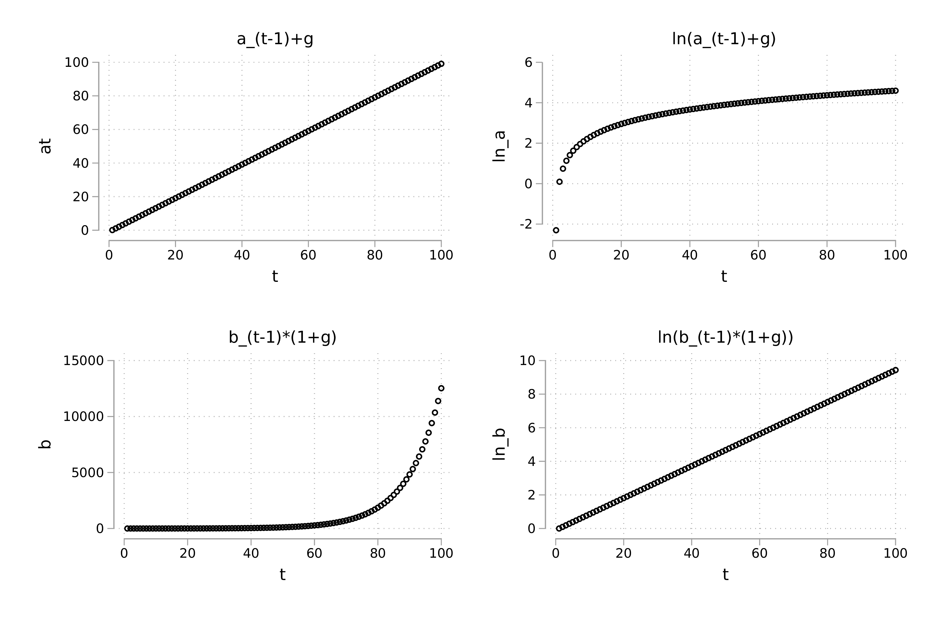
Solution to exercise 3.22: Investments over time

The formula under discrete time is: \[ Y_t=Y_0\cdot (1+g)^t \] The formula under continuous time is: \[ Y_t=Y_0\cdot e^{gt} \]

Solution to exercise 3.23: Exponential growth

Figure @ref(fig:expgrowth_graphs) provides the solution.

(#fig:expgrowth_graphs) Various growth functions

Solution to exercise 4.2: Derivation of demand function using the Lagrangian multiplier

The Lagrangian for this problem is \[ Z=x y+\lambda\left(P_{x} x+P_{y} y-B\right) \] The first order conditions are \[ \begin{array}{l} Z_{x}=y+\lambda P_{x}=0 \\ Z_{y}=x+\lambda P_{y}=0 \\ Z_{\lambda}=-B+P_{x} x+P_{y} y=0 \end{array} \]

Solving the first order conditions yield the following solutions

\[ x^{M}=\frac{B}{2 P_{x}} \quad y^{M}=\frac{B}{2 P_{y}} \quad \lambda=\frac{B}{2 P_{x} P_{y}} \] where \(x^{M}\) and \(y^{M}\) are the consumer’s demand functions.

Solution to exercise 4.3: Cobb-Douglas and demand

The Lagrangian is \[ \mathcal{L}(x, y)=A x^{\alpha} y^{\beta}+\lambda(p x+q y-I) \]

Therefore, the first-order conditions are \[ \begin{aligned} \mathcal{L}_{x}^{\prime}(x, y)=A \alpha x^{\alpha-1} y^{\beta}+\lambda p &=0 \qquad (*)\\ \mathcal{L}_{y}^{\prime}(x, y)=A x^{\alpha} \beta y^{\beta-1}+\lambda q &=0 \qquad (**)\\ p x+q y-I &=0 \qquad (***) \end{aligned} \]

Solving \((*)\) and \((**)\) for \(\lambda\) yields \[ \lambda=\frac{A \alpha x^{\alpha-1} y^{\beta-1} y}{p}=\frac{A x^{\alpha-1} x \beta y^{\beta-1}}{q} \] Canceling the common factor \(A x^{\alpha-1} y^{\beta-1}\) from the last two fractions gives \[ \frac{\alpha y}{p}=\frac{x \beta}{q} \] and therefore \[ q y=p x \frac{\beta}{\alpha} \] Inserting this result in \((***)\) yields \[ p x+p x \frac{\beta}{\alpha}=I \] Rearranging gives \[ p x\left(\frac{\alpha+\beta}{\alpha}\right)=I \] Solving for \(x\) yields the following \[ x=\frac{\alpha}{\alpha+\beta} \frac{I}{p} \] Inserting \[ p x=q y \frac{\alpha}{\beta} \] in \((***)\) gives \[ q y \frac{\partial}{\beta}+q y=I \] and therefore the \[ y=\frac{\beta}{\alpha+\beta} \frac{I}{q} \]

Solution to exercise 4.4: Understanding indifference curves and budget constraints

1. \(IC_3\) represents the highest level of utility. \(IC_1\) represents the lowest level of utility.
   
2. Task solved in class.
3. Task solved in class.
4. The budget line can be sketched into a y-x plot by solving \(p_xx+p_yy=I\) for y: \[y=\frac{I}{p_y}-\frac{p_x}{p_y}x\]

Solution to exercise 6.2: Isoquants

Graph (1) shows perfect complements and graph (2) perfect substitutes. The isoquants for Cobb-Douglas production functions is convex and in between the two extremes and it shifts outward with more production.

Solution to exercise 3.3: Labor and machines

1. Set up Lagrangian: \[\mathcal{L} = K^{0.4}L^{0.6} - 216\lambda + 2\lambda L + 8\lambda K\]
   
2. FOC: \[\begin{align*} 0 &= 0.4K^{-0.6}L^{0.6} - 8\lambda \quad (*) \\ 0 &= 0.6K^{0.4}L^{-0.4} - 2\lambda \quad (**) \\ 0 &= 216 - 2L - 8K \quad (***) \\ \end{align*}\]
3. Solving (*) and (**) for \(\lambda\) and substituting \(\lambda\) gives us: \[\frac{1}{6}L = K \quad (****)\]
4. Plugging (****) into (***) yields: \[0 = 216 - 2L - 8\cdot\left(\frac{1}{6}L\right) \Rightarrow L = 64\frac{4}{5}\]
5. Using that result in (***) again, we get: \[216 - 2\cdot 64\frac{4}{5} + 8K \Rightarrow K = 10\frac{4}{5}\]

Thus, the optimal combination of inputs is \(L = 64\frac{4}{5}\) and \(K = 10\frac{4}{5}\).

Solution to exercise 4.6: Marginal revenue and total revenue

See: chapter 15.2 Profit Maximization for Monopolists of Emerson (2019), see: here.

Solution to exercise 4.7: How to maximize profits

1. \(PED=\frac{17}{31} \approx 0.5483\)
2. The demand function can be derived using the point-slope formula and one sales point: \[P-40=-\frac{1}{10}(Q-800) \Rightarrow P=120-\frac{1}{10}Q \Rightarrow Q=1200-10P\]
3. Total costs (TC) are given by \(TC=FC+VC=FC+MC \cdot Q\). Solving the system of equations: \[26500=FC+750 \cdot MC\] \[28000=FC+800 \cdot MC\] we find \(MC=30\) and \(FC=4000\). The cost function is \(TC=4000+30 \cdot Q\).
4. The revenue function is given by \(TR=P \cdot Q(P)\). Plugging the demand function in gives: \[TR(Q)=120Q-\frac{1}{10}Q^2\]
5. The marginal revenue function is \(\frac{TR(Q)}{\partial Q}=120-\frac{2}{10}Q\).
6. The marginal cost function is \(MC=30\) (as found in step 3).
7. Setting \(MC=MR\), we find the optimal quantity: \[30=120-\frac{2}{10}Q \Rightarrow Q^*=450\] Plugging \(Q^*\) into the demand function, we find the optimal price: \(P^*=120-\frac{1}{10} \cdot 450 = 75\)
8. Profit (\(\pi\)) is given by \(\pi=TR-TC\): \[\pi_{t=1}=1200 \cdot 45-10 \cdot 45^2-4000-30 \cdot 750 = 7250\] \[\pi_{t=2}=1200 \cdot 40-10 \cdot 40^2-4000+30 \cdot 800 = 4000\] \[\pi_{t=3}=1200 \cdot 75-10 \cdot 75^2-4000+30 \cdot 450 = 16250\]

Solution to exercise 4.8: Agricultural land use

The maximum rent a farmer of a respective production method can offer is the rate where zero profit is made. The market rent curve of the landlord is the upper envelope: \(r(x) = \max(r_i(x))\), where the profit \(\pi\) and the rent \(r\) for firm \(i\) are given as follows:

\[ \pi_i = q_i(p_i - c_i - \theta_i x) - r_i(x) \] \[ r_i(x) = q_i(p_i - c_i - \theta_i x) \]

Bid rent curve	\(\frac{\partial r_i}{\partial x}\)	Intercept	Nullstelle
\(r_1 = 10(5 - 1 - 0.4x) = 40 - 4x\)	-4	40	10
\(r_2 = 5(5 - 2 - 0.1x) = 15 - 0.5x\)	-0.5	15	30
\(r_3 = 30(2 - 1 - 0.15x) = 30 - 4.5x\)	-4.5	30	6.67
\(r_4 = 20(6 - 5 - 0.05x) = 20 - x\)	-1	20	20

When plotting the corresponding market rent curve, it becomes apparent that regions 1, 4, and 2 dominate the market from the center. The market boundary points are determined as follows: \[ 40 - 4x_{14} = 20 - x_{14} \Longleftrightarrow x_{14} = \frac{20}{3} \] \[ 15 - 0.5x_{42} = 20 - x_{42} \Longleftrightarrow x_{42} = 10 \] This means that in the range \(x \in [0, \frac{20}{3}]\), land use form 1 prevails; in the range \(x \in [\frac{20}{3}, 10]\), land use form 4 prevails; and in the range \(x \in [10, 30]\), land use form 2 prevails.

Solution to exercise 6.1: Understanding production

1. Any point that lies either on the production possibilities curve or to the left of it is said to be an attainable point: it can be produced with currently available resources. Production points that lie in the yellow shaded area are said to be unattainable because they cannot be produced using currently available resources. These points represent an inefficient production, because existing resources would allow for production of more of at least one good without sacrificing the production of any other good. An efficient point is one that lies on the production possibilities curve. At any such point, more of one good can be produced only by producing less of the other.

2. The PPF would shift outwards.

3. The PPF would shift inwards.
   

4. The PPF would shift…

   1. …outwards for both goods.
   2. …inwards for good A, see figure 6.17.
   3. …outwards for good B.

5. With economies of scale, the PPF would curve inward, with the opportunity cost of one good falling as more of it is produced. A straight-line (linear) PPF reflects a situation where resources are not specialized and can be substituted for each other with no added cost. With constant returns to scale, there are two opportunities for a linear PPF: if there was only one factor of production to consider or if the factor intensity ratios in the two sectors were constant at all points on the production-possibilities curve.

6. Here is one example: Suppose a country that is endowed with two factors of production and that one factor can only be used for producing good A and the other factor can only be used to produce good B.

Shrinking production possibilities in good A

Solution to exercise 6.3: Calculate with log

• \(\log_2 16=4\) because \(2^4=16\)
• \(\log_3 243=5\) because \(3^5=243\)
• \(\log_5 125=3\) because \(5^3=125\)
• \(\log_3 81=4\) because \(3^4=81\)
• \(\log_2 \left(\frac{1}{8}\right)=-3\) because \(2^{-3}=\frac{1}{8}\)

6.4 Past exams

Please feel free to download a collection of past exams here.

---

21. Taken from https://de.wikipedia.org/wiki/Haus_vom_Nikolaus↩︎

22. Taken from https://de.wikipedia.org/wiki/Haus_vom_Nikolaus↩︎