3 Decision making theory
3.1 Decision making under certainty
After successful completion of the module, students are able to:
- Distinguish different theories of decision making.
- Calculate the optimal decision under certainty, uncertainty, and under risk.
- Describe and use various criteria of decision making.
- Simplify complex decision making situations and use formal approaches of decision making to guide the decision making behavior of managers.
- Avoid common mistakes when applying heuristics in decision making.
- Use investment calculus to make good financial decisions.
Decision making under certainty means that we assume that we are certain about the future state of nature, i.e., we have complete information about the alternative actions and their consequences. Making decisions under certainty may seem like a trivial exercise. However, many problems are so complex that sophisticated mathematical techniques are sometimes needed to find the best solution.
3.1.1 Decision making with complex state of natures
Suppose you have to decide between four different restaurants where you want to go out to eat (\(a_1\), \(a_2\), \(a_3\), \(a_4\)). The restaurants have different characteristics such as the quality of the food k1, the quality of the music played \(k_2\), the price \(k_3\), the quality of the service \(k_4\), and the environment \(k_5\). The corresponding payoff table is given below. High numbers represent good quality. In other words, \(a_i\) refer to competing alternatives where to eat for dinner, and \(k_i\) are certain characteristics of the respective restaurant, and the numbers given in the table indicate the output.
| \(k_1\) | \(k_2\) | \(k_3\) | \(k_4\) | \(k_5\) | |
|---|---|---|---|---|---|
| \(a_1\) | 3 | 0 | 7 | 1 | 4 |
| \(a_2\) | 4 | 1 | 4 | 2 | 1 |
| \(a_3\) | 4 | 0 | 3 | 2 | 1 |
| \(a_4\) | 5 | 1 | 2 | 3 | 1 |
Domination
Some alternative can be excluded because they are dominated by other alternatives. In the scheme above you can see that alternative 2 is always superior to alternative 3, i.e., alternative 3 is dominated by alternative 2. Thus, it does not make sense to think about alternative 3:
| \(k_1\) | \(k_2\) | \(k_3\) | \(k_4\) | \(k_5\) | |
|---|---|---|---|---|---|
| \(a_1\) | 3 | 0 | 7 | 1 | 4 |
| \(a_2\) | 4 | 1 | 4 | 2 | 1 |
| \(a_3\) | |||||
| \(a_4\) | 5 | 1 | 2 | 3 | 1 |
Weighting
As the objectives \(k_j\) of the scheme above do not represent different states of nature but represent characteristics and its corresponding utility (whatever that number may mean in particular) of one particular characteristics if we choose a respective alternative. For example, think of that you can choose one out of four restaurants, \(a_1,\dots,a_4\), in order to eat a five-course menu, \(k_1,\dots,k_5\), and the outcome represents your utility of each course, \(j\), for each restaurant, \(i\). We already know from the domination principle that restaurant \(a_3\) is a bad choice.
Suppose you have a preference for the first three courses. Specifically, suppose that your preference scheme is as follows:
\[ g_1 : g_2 : g_3 : g_4 : g_5 = 3 : 4 : 3 : 1 : 1 \]
This means, for example, that you value the second food course four times more than the last course.
\[ w_1=3/12; w_2=4/12; w_3=3/12; w_4 = w_5 =1/12. \]
In order to find a decision criteria you can calculate the aggregated expected utility as follows:
\[ \Phi(a_i)=\sum_{p=1}^{r}w_p\cdot u_{ip} \rightarrow max \]
The results are as follows:
| \(k_1\) | \(k_2\) | \(k_3\) | \(k_4\) | \(k_5\) | \(\Phi(a_i)\) | |
|---|---|---|---|---|---|---|
| \(a_1\) | 3 | 0 | 7 | 1 | 4 | 35//12 |
| \(a_2\) | 4 | 1 | 4 | 2 | 1 | 31//12 |
| \(a_3\) | 4 | 0 | 3 | 2 | 1 | 24//12 |
| \(a_4\) | 5 | 1 | 2 | 3 | 1 | 29//12 |
Thus, \(a_1\succ a_2 \succ a_4 \succ a_3\), i.e., you prefer alternative \(a_1\).
Preferences and decision criteria
Maybe not all courses play the same role for you so you can take your decision based on your preference scheme. For example, assume some courses are more important to you than others such as \(k_1 \succ k_3 \succ k_2 \succ k_4 \succ k_5\). Now, if you decide based on your most important course you should choose restaurant 4 because this gives you the highest utility in that dish. If you further assume that you are not that hungry and you only like to have two dishes, then you should probably better go for restaurant 1 because the aggregated utility in the two preferred courses is 10 utility units and restaurants 2, 3 and 4 can only offer 8, 7 and 7 utility units in your two preferred courses.
Körth’s Maximin-Rule
According to this rule, we compare alternatives by the worst possible outcome under each alternative, and we should choose the one which maximizes the utility of the worst outcome. More concrete, the procedure consists of 4 steps:
- Calculate the utility maximum for each column \(j\) of the payoff matrix: \[\overline{O}_j=\max_{i=1,\dots,m}{O_{ij}}\qquad \forall j.\]
- Calculate for each cell the relative utility, \[\frac{O_{ij}}{\overline{O}_j}.\]
- Calculate for each row \(i\) the minimum: \[\Phi(a_i)=\min_{j=1,\dots,p}\left(\frac{O_{ij}}{\overline{O}_j}\right) \qquad \forall i.\]
- Set preferences by maximizing \(\Phi(a_i)\).
3.1.2 Linear programming
Linear Programming is a common technique for decision making under certainty. It allows to express a desired benefit (such as profit) as a mathematical function of several variables. The solution is the set of values for the independent variables (decision variables) that serves to maximize the benefit or to minimize the negative outcome under consideration of certain limits, a.k.a. constraints. The method usually follows a four step procedure:
- state the problem;
- state the decision variables;
- set up an objective function;
- clarify the constraints.
Example: Consider a factory producing two products, product X and product Y. The problem is this: If you can realize $10.00 profit per unit of product X and $14.00 per unit of product Y, what is the production level of x units of product X and y units of product Y that maximizes the profit P each day? Your production, and therefore your profit, is subject to resource limitations, or constraints. Assume in this example that you employ five workers—three machinists and two assemblers—and that each works only 40 hours a week.12
- Product X requires three hours of machining and one hour of assembly per unit.
- Product Y requires two hours of machining and two hours of assembly per unit.
- State the problem: How many of product X and product Y to produce to maximize profit?
- Decision variables: Suppose x denotes the number of product X to produce per day and y denotes number of product Y to produce per day
- Objective function: Maximize \[P = 10x + 14y\]
- Constraints:
- machine time=120h
- assembling time=80h
- hours needed for production of one good:
machine time: \(x\rightarrow 3h\) and \(y \rightarrow 2h\)
assembling time: \(x\rightarrow 1h\) and \(y \rightarrow 2h\)
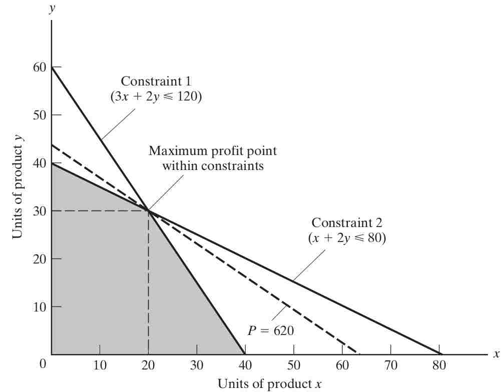
Thus, we get: \[3x + 2y \leq 120 \quad \Leftrightarrow y\leq 60-\frac{3}{2}x \quad \text{(hours of machining time)}\] \[x + 2y \leq 80 \quad \Leftrightarrow y \leq 40-\frac{1}{2}x \quad \text{(hours of assembly time)}\] Since there are only two products, these limitations can be shown on a two-dimensional graph (3.1). Since all relationships are linear, the solution to our problem will fall at one of the corners.
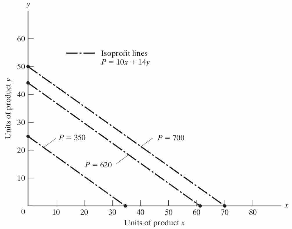
To draw the isoprofit function in a plot with the good \(y\) on the y-axis and good \(x\) on the x-axis, we can re-arrange the objective function to get \[y=\frac{1}{14}P-\frac{10}{14}x\] To illustrate the function let us consider some arbitrarily chosen levels of profit in :
- $350 by selling 35 units of X or 25 units of Y
- $700 by selling 70 units of X or 50 units of Y
- $620 by selling 62 units of X or 44.3 units of Y.
To find the solution, begin at some feasible solution (satisfying the given constraints) such as \((x,y) = (0,0)\), and proceed in the direction of steepest ascent of the profit function (in this case, by increasing production of Y at $14.00 profit per unit) until some constraint is reached. Since assembly hours are limited to 80, no more than 80/2, or 40, units of Y can be made, earning \(40 \cdot \$14.00\), or $560 profit. Then proceed along the steepest allowable ascent from there (along the assembly constraint line) until another constraint (machining hours) is reached. At that point, (x,y) = (20,30) and profit P = (20 * +10.00) + (30 * +14.00), or $620. Since there is no remaining edge along which profit increases, this is the optimum solution.
Exercise 3.1 Körth: example
For the following payoff-matrix, calculate the order of preferences based on the Körth-rule.
| \(O_{ij}\) | \(k_1\) | \(k_2\) | \(k_3\) | \(k_4\) | \(k_5\) |
|---|---|---|---|---|---|
| \(a_1\) | 3 | 0 | 7 | 1 | 4 |
| \(a_2\) | 4 | 0 | 4 | 2 | 1 |
| \(a_3\) | 4 | -1 | 3 | 2 | 1 |
| \(a_4\) | 5 | 1 | 3 | 3 | 1 |
Please find solution to the exercise in the appendix.
3.1.3 Lagrange multiplier method
The method outlined below requires an understanding of how to take derivatives of functions and solve systems of equations. If readers feel they need a refresher on these topics, I recommend consulting the lecture notes Calculus and Linear Algebra from Huber (2023).
The decision-making process of consumers and producers lies at the core of microeconomic research and is of significant importance for managers. I will not go into detail here, but I will show some examples of how to come to a decision when certain information is given.
Before we come to the Lagrangian multplier method, let me define what (micro)economist mean when they speak of firms and consumers.
A firm is a productive unit. In particular, it is an organization that produces goods and services, called the output. To do so, it uses inputs called factors of production: labor, capital, land, skills, etc. The relationship between the inputs and the output is the production function. The goal of the firm is to achieve whatever goal its owner(s) decide to achieve. Usually, it is (and in Germany, for example, it has to be the case by law) to generate profits, i.e., total revenue minus total cost for the level of production. Determining the optimal level of production for a firm is a multifaceted decision that encompasses various strategic aspects and is heavily influenced by the market situation of firms. This includes factors such as market power, demand function, production function, cost function, and revenue function.
A consumer is an individual that purchases goods or services to satisfy their needs. They make decisions regarding what to buy, how much to buy in order to maximize their utility. Microeconomists study consumer behavior and factors that influence it, such as prices, income, preferences, and market conditions, to understand the choices consumers make and their impact on markets and the overall economy.
For a deeper understanding of the microeconomic preliminaries related to this topic, please read section 6.1 of the appendix.
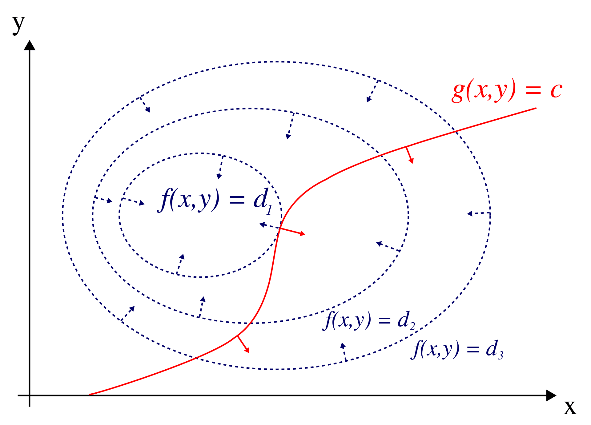
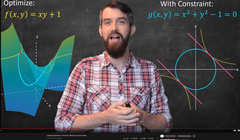
The Lagrange multiplier method, named after Joseph-Louis Lagrange, is a strategy for finding the local maxima and minima of a function subject to constraints. The red curve in Figure 3.4 represents the constraint \(g(x, y) = c\), while the blue curves depict contours of \(f(x, y)\). The point where the red constraint tangentially intersects a blue contour represents the maximum of \(f(x, y)\) along the constraint, as \(d1 > d2\).
For a detailed visual explanation of the method, you can watch Dr. Trefor Bazett’s YouTube video on Lagrange Multipliers | Geometric Meaning & Full Example, see figure 3.5.
The Lagrange multiplier method, named after Joseph-Louis Lagrange, is a powerful technique for solving optimization problems with constraints. It allows us to find the local maxima and minima of a function subject to certain conditions. The method involves four key steps:
Step 1: Formulate the Problem
Define the problem you want to solve in mathematical terms. This includes specifying the objective function to be maximized or minimized and the constraints that need to be satisfied.
The problem that we want to solve can be written in the following way, \[ \begin{array}{ll} \max _{x, y} & F(x, y) \\ \text{ s.t. } & g(x, y)=0 \end{array} \] where \(F(x, y)\) is the function to be maximized and \(g(x, y)=0\) is the constraint to be respected. Notice that \(\max _{x, y}\) means that we must solve (maximize) with respect to \(x\) and \(y\).
Step 2: Construct the Lagrangian
Create a new function called the Lagrangian by combining the objective function and the constraints using Lagrange multipliers. The Lagrangian introduces new variables, known as Lagrange multipliers, to account for the constraints. The Lagrangian, \(\mathcal{L}\), is a combination of the functions that explain the problem: The \(\lambda\) is called the Lagrange Multiplier. \[ \mathcal{L}(x, y, \lambda)=F(x, y)-\lambda g(x, y) \]
Step 3: Determine the First-Order Conditions
Differentiate the Lagrangian with respect to the variables of the problem (e.g., x and y) and the Lagrange multipliers. Set the partial derivatives equal to zero to obtain the first-order conditions. These conditions represent the necessary conditions for optimality.
Differentiate \(\mathcal{L}\) w.r.t. \(x, y,\) and \(\lambda\) and equate the partial derivatives to 0: \[\begin{align*} \frac{\partial \mathcal{L}(x, y, \lambda)}{\partial x}=0 & \Leftrightarrow \frac{\partial F(x, y)}{\partial x}-\lambda \frac{\partial g(x, y)}{\partial x}=0 \\ \frac{\partial \mathcal{L}(x, y, \lambda)}{\partial y}=0 & \Leftrightarrow \frac{\partial F(x, y)}{\partial y}-\lambda \frac{\partial g(x, y)}{\partial y}=0 \\ \frac{\partial \mathcal{L}(x, y, \lambda)}{\partial \lambda}=0 & \Leftrightarrow g(x, y)=0 \end{align*}\]
Step 4: Solve the System of Equations
Solve the system of equations obtained from the first-order conditions to find the values of the variables and Lagrange multipliers that satisfy the optimality conditions. The solutions represent the optimal quantities that maximize or minimize the objective function subject to the given constraints.
By following these four steps, you can effectively apply the Lagrange multiplier method to various optimization problems with constraints. It provides a systematic approach to finding the optimal solutions while incorporating the necessary trade-offs imposed by the constraints.
Exercise 3.2 Burgers and drinks
Suppose you are in a fast food restaurant and you want to buy burgers and some drinks. You have €12 to spend, a burger costs €3 and a drink costs €2.
- Assume that you want to spend all your money and that you can only buy complete units of each products. What are the possible choices of consumption?
- Given your utility function \(U(x,y)=B^{0.6}D^{0.4}\) calculate for each possible consumption point your overall utility. How will you decide?
- Assume that you want to spend all your money and that both products can be bought on a metric scale where one burger weights 200 grams and a drink is 200 ml. How much of both goods would you consume now? Hint: Use the Lagrangian multiplier method.15
Please find solution to the exercise in the appendix.
Exercise 3.3 Labor and machines
Suppose you rent a factory for a month to produce as many masks as possible. After you have paid the rent, you need to decide how many machines to buy and how many workers to hire for the given month.
What is the optimal amount of workers and machines to employ for the given month, if you assume the following:
- \(L\) denotes the number of workers
- \(K\) denotes the number of machines
- \(Q\) denotes the number of masks produced
- \(p_L\) denotes the price of a worker for a month
- \(p_K\) denotes the price of a machine for a month
- \(B\) denotes the money you can invest in the production of masks for the next month
- \(B = 216\)
- The production of masks can be explained by the following Cobb-Douglas production function: \(Q = K^{0.4}L^{0.6}\)
- \(p_L = 2\)
- \(p_K = 8\)
Please find solution to the exercise in the appendix.
Exercise 3.4 Consumption choice
Suppose you want to spend your complete budget of €30, \[I=30,\] on the consumption of two goods, \(A\) and \(B\). Further assume good \(A\) costs €6, \[p_A=6,\] and good \(B\) costs €4, \[p_B=4\] and that you want to maximize your utility that stems from consuming the two goods. Calculate how much of both goods to buy and consume, respectively, when your utility function is given as \[U(A,B)=A^{0.8}B^{0.2}\]
Please find solution to the exercise in the appendix.
Exercise 3.5 Cost-minimizing combination of factors
Using two input factors \(r_1\) and \(r_2\), a firm wants to produces a fixed quantity of a product, that is \(x=20\). Given the production function \[ x=\frac{5}{4} r_1^{\frac{1}{2}} r_2^{\frac{1}{2}} \] and the factor prices \[ p_{r_1}=1 \quad \text{ and } p_{r_2}=4. \] calculate the cost-minimizing combination of factors (\(r_1, r_2\)).
Please find solution to the exercise in the appendix.
Exercise 3.6 Lagrange with n-constraints
Write down the Lagrangian multiplier for the following minimization problem:
Minimize \(f(\mathbf{x})\) subject to: \[\begin{aligned} g_1(\mathbf{x})&=0 \\ g_2(\mathbf{x})&=0\\ &\vdots\\ g_n(\mathbf{x})&=0,\end{aligned}\] where \(n\) denotes the number of constraints.
Please find solution to the exercise in the appendix.
3.2 Decision making under uncertainty
When it comes to decision-making under uncertainty you need to have a criterion that helps you to come to a rational decision. The choice of criteria is a matter of taste and should at best fit with overall (business) strategy.
Laplace criterion
In case of different possible states of nature and no information on their probability of occurrences, the Laplace criterion simply assigns equal probabilities to the possible pay offs for each action and then selecting that alternative which corresponds to the maximum expected pay off. An example is given in Finne (1998).
Maximax criterion (go for cup)
If you like to go for cup, i.e., like to have the best out of the best possible outcome without taking into consideration the fact that this may potentially also result in the worst possible scenario, then, you can choose the alternative that gives the maximum possible output.
Minimax criterion (best of the worst)
The Minimax (or maximin) criterion is a conservative criterion because it is based on making the best out of the worst possible conditions. Again, examples on how to calculate it are given in Finne (1998)..
Savage Minimax criterion
This criterion aims to minimize the worst-case regret to perform as closely as possible to the optimal course. Since the minimax criterion applied here is to the regret (difference or ratio of the payoffs) rather than to the payoff itself, it is not as pessimistic as the ordinary minimax approach. For more details, please read Finne (1998).
Hurwicz criterion
The Hurwicz criterion allows the decision maker to calculates a weighted average between the best and worst possible payoff for each decision alternative. Then, the alternative with the maximum weighted average is chosen.
For each decision alternative, the weight \(\alpha\) is used to compute Hurwicz the value: \[H_i=\alpha \cdot \overline{O}_i + (1-\alpha)\cdot \underline{O}_i\] where \(\overline{O}_i=\max_{j=1,\dots,p}{O_{ij}}\qquad \forall i\) and \(\underline{O}_i=\min_{j=1,\dots,p}{O_{ij}}\qquad \forall i\), i.e., the respective maximum and minimum Output for each alternative, \(i\). The example that is shown in Figure 7 of Finne (1998, p. 401) contains some errors. Here is the correct table including the Hurwicz-values (we assume a \(\alpha=.5\)):
| \(O_{ij}\) | \(min(\theta_1)\) | \(max(\theta_2)\) | \(H_i\) |
|---|---|---|---|
| \(a_1\) | 36 | 110 | 73 |
| \(a_2\) | 40 | 100 | 70 |
| \(a_3\) | 58 | 74 | 66 |
| \(a_4\) | 61 | 66 | 63.5 |
Thus, the order of preference is \(a_4\succ a_3 \succ a_1 \succ a_2\).
Exercise 3.7 Three categories
Read Finne (1998) and answer the following questions:
- Explain the three categories of decision making.
- Give examples of the three categories of decision making.
- Explain the four criteria for decision making under uncertainty.
3.3 Decision making under risk
When some information is given about the probability of occurrence of states of nature, we speak of decision-making under risk. The most straight forward technique to make a decision here is to maximize the expected outcome for each alternative given the probability of occurrence, \(p_j\).
However, the expected utility hypothesis states that the subjective value associated with an individual’s gamble is the statistical expectation of that individual’s valuations of the outcomes of that gamble, where these valuations may differ from the Euro value of those outcomes. Thus, you should better look on the utility of a respective outcome rather than on the outcome itself because the utility and outcome do not have to be linked in a linear way. The St. Petersburg Paradox by Daniel Bernoulli in 1738 is considered the beginnings of the hypothesis.
3.3.1 St. Petersburg Paradox
3.3.1.1 Ininite St. Petersburg lotteries
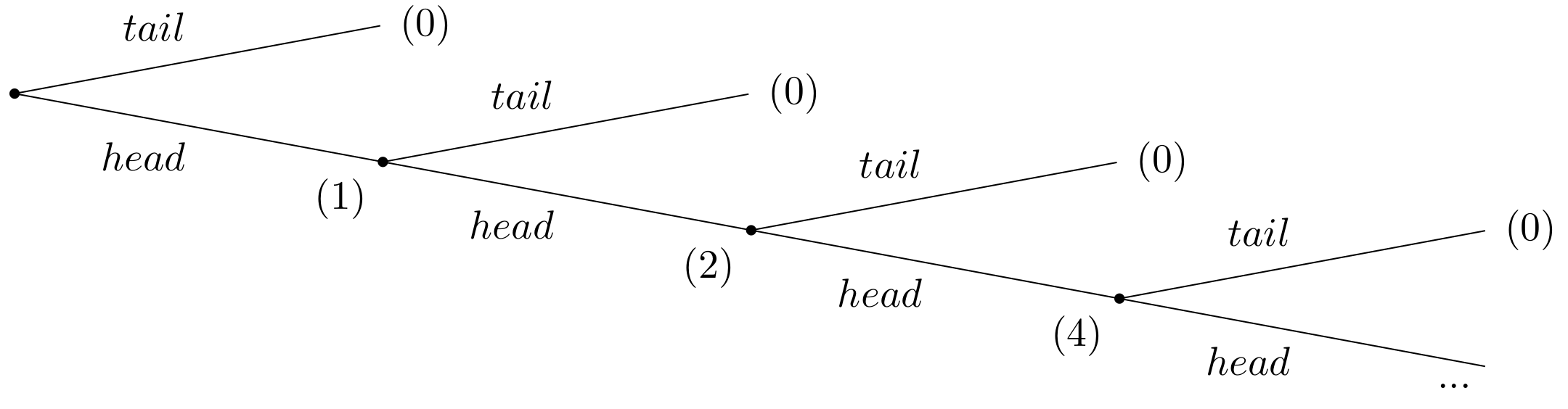
Suppose a casino offers a game of chance for a single player, where a fair coin is tossed at each stage. The first time head appears the player gets $1. From then onwards, every time a head appears, the stake is doubled. The game continues until the first tails appears, at which point the player receives \(\$ 2^{k-1}\), where k is the number of tosses (number of heads) plus one (for the final tails). For instance, if tails appears on the first toss, the player wins $0. If tails appears on the second toss, the player wins $2. If tails appears on the third toss, the player wins $4, and so on. The extensive form of the game is given in figure 3.6.
Given the rules of the game, what would be a fair price for the player to pay the casino in order to enter the game?
To answer this question, one needs to consider the expected payout: The player has a 1/2 probability of winning $1, a 1/4 probability of winning $2, a 1/8 probability of winning $4, and so on. Thus, the overall expected value can be calculated as follows: \[ E = \frac{1}{2} \cdot 1 + \frac{1}{4} \cdot 2 + \frac{1}{8} \cdot 4+ \frac{1}{16} \cdot 8 + \dots \] This can be simplified as: \[ E = \frac{1}{2} + \frac{1}{2} + \frac{1}{2} + \frac{1}{2} + \dots = + \infty. \] That means the expected win for playing this game is an infinite amount of money. Based on the expected value, a risk-neutral individual should be willing to play the game at any price if given the opportunity. The willingness to pay of most people who have given the opportunity to play the game deviates dramatically from the objectively calculable expected payout of the lottery. This describes the apparent paradox.
In the context of the St. Petersburg Paradox, it becomes evident that relying solely on expected values is inadequate for certain games and for making well-informed decisions. Expected utility, on the other hand, has been the prevailing concept used to reconcile actual behavior with the notion of rationality thus far.
Finite St. Petersburg lotteries
Let us assume that at the beginning, the casino and the player agrees upon how many times the coin will be tossed. So we have a finite number I of lotteries with \(1 \leq I \leq \infty\).
To calculate the expected value of the game, the probability \(p(i)\) of throwing any number \(i\) of consecutive head is crucial. This probability is given by \[ p(i)=\underbrace{\frac{1}{2} \cdot \frac{1}{2} \cdot \cdots \frac{1}{2}}_{i \text { factors}}=\frac{1}{2^{i}} \] The payoff \(W(I)\) is, if head appears \(I\)-times in a row by \[ W(I)=2^{I-1} \] The expected payoff \(E(W(I))\) if the coin is flipped \(I\) times is then given by \[ E(W(I))=\sum_{i=1}^{I} p(i) \cdot W(i)=\sum_{i=1}^{I} \frac{1}{2^{i}} \cdot 2^{i-1}=\sum_{i=1}^{I} \frac{1}{2}=\frac{I}{2} \]
Thus, the expected payoff grows proportionally with the maximum number of rolls. This is because at any point in the game, the option to keep playing has a positive value no matter how many times head has appeared before. Thus, the expected value of the game is infinitely high for an unlimited number of tosses but not so for a limited number of tosses. Even with a very limited maximum number of tosses of, for example, \(I = 100\), only a few players would be willing to pay $50 for participation. The relatively high probability to leave the game with no or very low winnings leads in general to a subjective rather low evaluation that is below the expected value.
In the real world, we understand that money is limited and the casino offering this game also operates within a limited budget. Let’s assume, for example, that the casino’s maximum budget is $20,000,000. As a result, the game must conclude after 25 coin tosses because \(2^{25} = 33,554,432\) would exceed the casino’s financial capacity. Consequently, the expected value of the game in this scenario would be significantly reduced to just $12.50. Interestingly, if you were to ask people, most would still be willing to pay less than $12.50 to participate. How can we explain this? Well, it is not the expected outcome that matters but the utility that stems from the outcome.
3.3.1.2 The impact of output on utility matters
Daniel Bernoulli (1700 - 1782) worked on the paradox while being a professor in St. Petersburg. His solution builds on the conceptual separation of the expected payoff and its utility. He describes the basis of the paradox as follows:
``Until now scientists have usually rested their hypothesis on the assumption that all gains must be evaluated exclusively in terms of themselves, i.e., on the basis of their intrinsic qualities, and that these gains will always produce a utility directly proportionate to the gain.’’ (Bernoulli, 1954, p. 27)
The relationship between gain and utility, however, is not simply directly proportional but rather more complex. Therefore, it is important to evaluate the game based on expected utility rather than just the expected payoff. \[ E(u(W(I)))=\sum_{i=1}^{I} p(i) \cdot u(W(i))=\sum_{i=1}^{I} \frac{1}{2^{i}} \cdot u\left(2^{i-1}\right) \] Daniel Bernoulli himself proposed the following logarithmic utility function: \[ u(W)=a \cdot \ln (W), \] where \(a\) is a positive constant. Using this function in the expected utility, we get \[ E(u(W(I)))=\sum_{i=1}^{I} \frac{1}{2^{i}} \cdot a \cdot \ln \left(2^{i-1}\right)=a \cdot \sum_{i=1}^{I} \frac{i-1}{2^{i}} \ln 2=a \cdot \ln 2 \cdot \sum_{i=1}^{I} \frac{i-1}{2^{i}}. \] The infinite series, \(\sum_{i=1}^{I} \frac{i-1}{2^{i}}\), converges to 1 (\(\lim _{I \rightarrow \infty} \sum_{i=1}^{I} \frac{i-1}{2^{i}}=1\)). Thus, given an ex ante unbounded number of throws, the expected utility of the game is given by \[ E(u(W(\infty)))=a \cdot \ln 2 . \]
In experiments in which people were offered this game, their willingness to pay was roughly between 2 and 3 Euro. Thus, the suggests logarithmic utility function seems to be a pretty realistic specification. The main reason is mathematically that the increasing expected payoff has decreasing marginal utility and hence the utility function reflects the risk aversion of many people.
Exercise 3.8 Rationality and risk
There are 90 balls in an box. It is known that 30 of them are red, the remaining 60 are blue or green. An individual can choose between the following lotteries:
| Payoff | probability | |
|---|---|---|
| Lottery 1 | 100 Euro if a red ball is drawn 0 Euro else | \(p=\frac{1}{3}\) |
| Lottery 2 | 100 Euro if a blue ball is drawn 0 Euro else | \(0 \leq p \leq \frac{2}{3}\) |
In a second variant it has the choice between the following lotteries:
| Payoff | probability | |
|---|---|---|
| Lottery 3 | 100 Euro if a red or green ball is drawn or 0 Euro else | \(\frac{1}{3} \leq p \leq 1\) |
| Lottery 4 | 100 Euro if a blue or green ball is drawn or 0 Euro else | \(p=\frac{2}{3}\) |
- Which of the lotteries does the individual choose on the basis of expected values (risk neutral)?
- Which of the lotteries does the individual choose on the basis of expected utility if the utility of a payoff of \(x\) is given by \(u(x) = x^2\)?
- Empirical studies, e.g. , show, however, that most individuals will usually choose lotteries 1 and 4. will. Discuss: Is this consistent with rational behavior?
3.4 Decision making with conditional probabilities (Bayes’ theorem)
After successful completion of the module, students are able to:
- Understand and use the terminology of probability.
- Determine whether two events are mutually exclusive and whether two events are independent.
- Calculate probabilities using the addition rules and multiplication rules.
- Calculate with conditional probabilities using Bayes Theorem.
- Construct and interpret venn and tree diagrams.
- Apply their knowledge of probability theory to decision making in business.
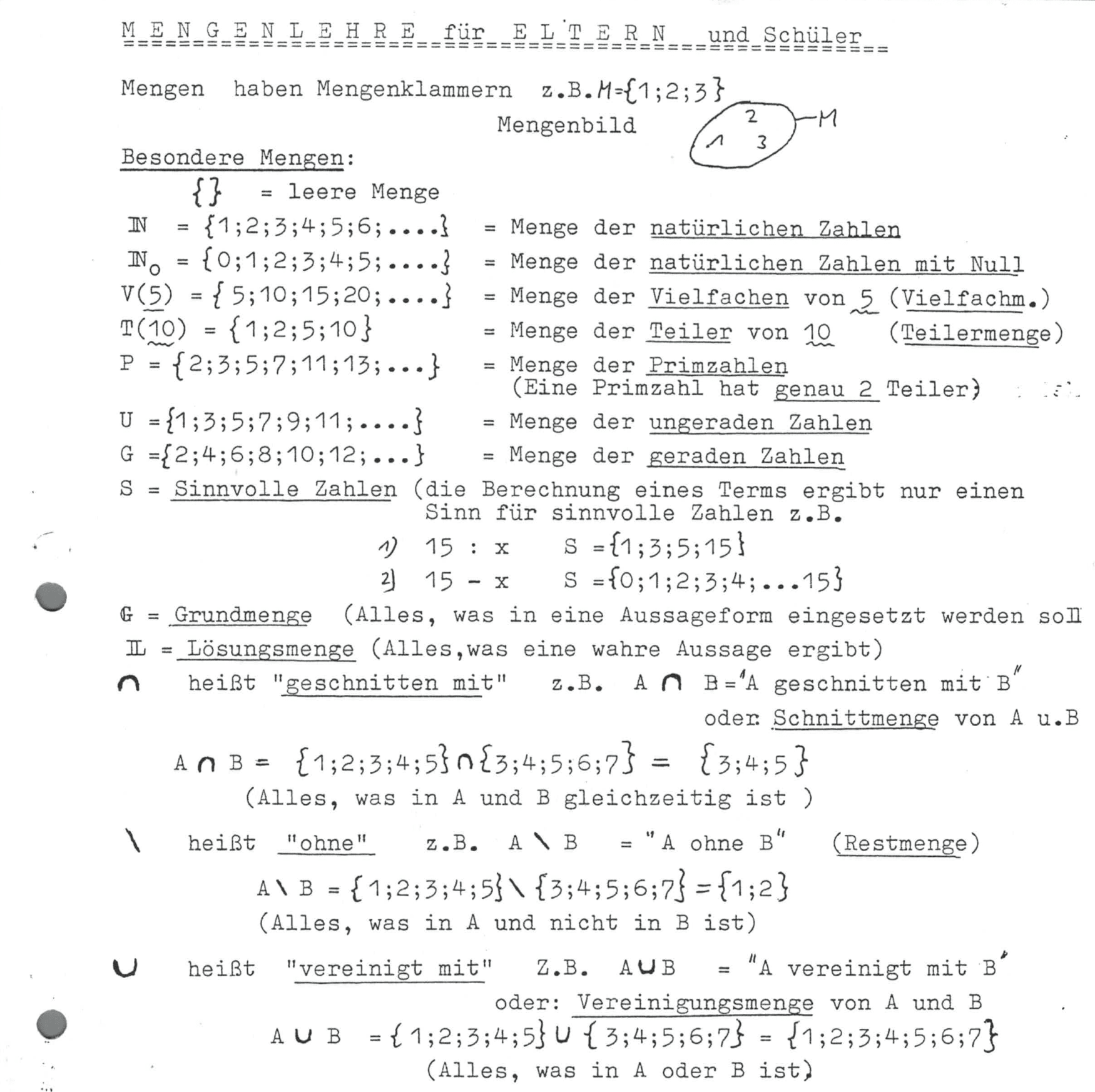
School Stuff
The next chapter will deal with stochastics. In Germany, stochastics is taught in the Gymnasium. If you are not from Germany, it was probably also part of your school experience. When I moved to Cologne in 2020, I found the following page shown in figure 3.10 that I had received from my high school math teacher. It was September 1993 and I was a desperate fifth grader in my fourth week. Perhaps you’d like to share your experiences with stochastics?
3.4.1 Terminology: \(P(A)\), \(P(A|B)\), \(\Omega\), \(\cap\), \(\neg\), …
3.4.1.1 Sample space
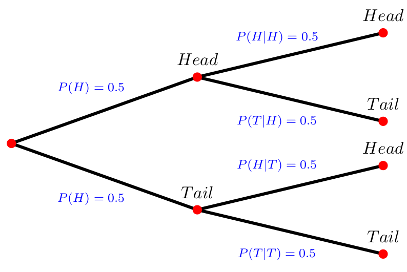
A result of an experiment is called an outcome. An experiment is a planned operation carried out under controlled conditions. Flipping a fair coin twice is an example of an experiment. The sample space of an experiment is the set of all possible outcomes. The Greek letter \(\Omega\) is often used to denote the sample space. For example, if you flip a fair coin, \(\Omega = \{H, T\}\) where the outcomes heads and tails are denoted with \(H\) and \(T\), respectively.
Example: Sample space Find the sample space for the following experiments:
- One coin is tossed.
- Two coins are tossed once.
- Two dices are tossed once.
- Picking two marbles, one at a time, from a bag that contains many blue, \(B\), and red marbles, \(R\).
Solutions:
- \(\Omega = \{head, tail\}\)
- \(\Omega = \{(head, head), (tail, tail),(head, tail),(tail, head)\}\)
- Overall, 36 different outcomes: \(\{ (1,1),(1,2),(1,3),(1,4),(1,5),(1,6),(2,1),(2,2),\dots,(6,6) \}\)
- \(\Omega = \{(B,B), (B,R), (R,B), (R,R)\}\).
Overall, there are three ways to represent a sample space:
- to list the possible outcomes (see example above),
- to create a tree diagram (see 3.11), or
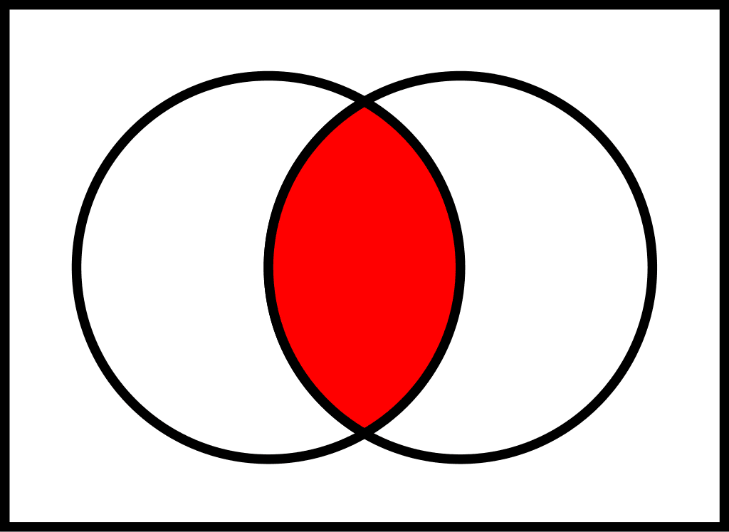
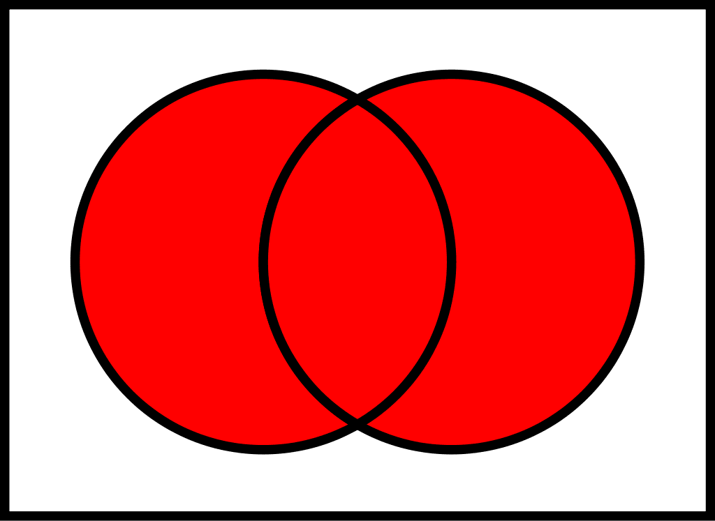
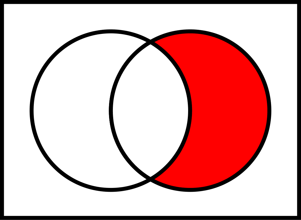
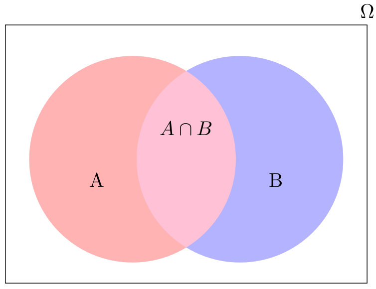
- to create a Venn diagram (see 3.12).
3.4.1.2 Probability
Probability is a measure that is associated with how certain we are of outcomes of a particular experiment or activity. The probability of an event \(A\), written \(P(A)\), is defined as \[ P(A)=\frac{\text{Number of outcomes favorable to the occurrence of } A}{\text{Total number of equally likely outcomes}}=\frac{n(A)}{n(\Omega)} \] For example, A dice has 6 sides with 6 different numbers on it. In particular, the set of elements of a dice is \(M=\{1,2,3,4,5,6\}\). Thus, the probability to receive a 6 is 1/6 because we look for one wanted outcome in six possible outcomes.
Example: Probability
When a fair dice is thrown, what is the probability of getting
- the number 5,
- a number that is a multiple of 3,
- a number that is greater than 6,
- a positive number that is less than 7.
Solutions: A fair dice is an unbiased dice where each of the six numbers is equally likely to turn up. The sample space is \(\Omega = \{1, 2, 3, 4, 5, 6\}\).
- Let A be the event of getting the number 5, \(A=\{5\}\). Then, \(P(A)=\frac{1}{6}\).
- Let \(B\) be the event of getting a multiple of 3, \(B=\{3, 6\}\). Then, \(P(B)=\frac{1}{3}\).
- Let \(C\) be the event of getting a number greater than 6, \(C=7,8,\dots\). Then, \(P(C)=0\) as there is no number greater than 6 in the sample space \(\Omega=\{1,2,3,4,5,6\}\). A probability of 0 means the event will never occur.
- Let D be the event of getting a number less than 7, \(D=\{1,2,3,4,5,6\}\). Then, \(P=1\) as the event will always occur.
3.4.1.3 The complement of an event (\(\neg-Event\))
The complement of event \(A\) is denoted with a \(\neg A\) or sometimes with a superscript `c’ like \(A^c\). It consists of all outcomes that are not in \(A\). Thus, it should be clear that \(P(A) + P(\neg A) = 1\). For example, let the sample space be \(\Omega = \{1, 2, 3, 4, 5, 6\}\) and let \(A = \{1, 2, 3, 4\}\). Then, \(\neg A = \{5, 6\}\); \(P(A) = \frac{4}{6}\); \(P(\neg A) = \frac{2}{6}\); and \(P(A) + P(\neg A) = \frac{4}{6}+\frac{2}{6} = 1\).
3.4.1.4 Independent events (AND-events)
Two events are independent when the outcome of the first event does not influence the outcome of the second event. For example, if you throw a dice and a coin, the number on the dice does not affect whether the result you get on the coin. More formally, two events are independent if the following are true: \[\begin{align*} P(A|B) &= P(A)\\ P(B|A) &= P(B)\\ P(A \cap B) &= P(A)P(B) \end{align*}\]
To calculate the probability of two independent events (\(X\) and \(Y\)) happen, the probability of the first event, \(P(X)\), has to be multiplied with the probability of the second event, \(P(Y)\): \[ P(X \text{ and } Y)=P(X \cap Y)=P(X)\cdot P(Y),\] where \(\cap\) stands for `and’. For example, let \(A\) and \(B\) be \(\{1, 2, 3, 4, 5\}\) and \(\{4, 5, 6, 7, 8\}\), respectively. Then \(A \cap B = \{4, 5\}\).
Example: Three dices
Suppose you have three dice. Calculate the probability of getting three times a 4.
Solutions: The probability of getting a \(4\) on one dice is 1/6. The probability of getting three \(4\) is: \[ P(4 \cap 4 \cap 4) = \frac{1}{6}\cdot \frac{1}{6}\cdot \frac{1}{6}= \frac{1}{216} \]
3.4.1.5 Dependent events (\(|\)-Events)
Events are dependent when one event affects the outcome of the other. If \(A\) and \(B\) are dependent events then the probability of both occurring is the product of the probability of \(A\) and the probability of \(A\) after \(B\) has occurred:
\[\begin{align*}
P(A \cap B)&=P(A)\cdot P(B|A),\\
\Leftrightarrow P(B|A)&=\frac{P(A \cap B)}{P(A)}\cdot
\end{align*}\]
where \(|A\) stands for after A has occurred', orgiven A has occurred’. In other words, \(P(B|A)\) is the probability of \(B\) given \(A\). This equation is also known as the Multiplication Rule.
The conditional probability of A given B is written \(P(A|B)\). \(P(A|B)\) is the probability that event A will occur given that the event B has already occurred. A conditional reduces the sample space. We calculate the probability of A from the reduced sample space B. The formula to calculate \(P(A|B)\) is \[ P(A|B) = \frac{P\left(A\cap B\right)}{P\left(B\right)}\] where \(P(B)\) is greater than zero. This formula is also known as Bayes’ Theorem, which is a simple mathematical formula used for calculating conditional probabilities, states that \[ P(A)P(B|A)=P(B)P(A|B) \] This is true since \(P(A \cap B)=P(B \cap A)\) and due to the fact that \(P(A\cap B)=P(B\mid A)P(A)\), we can write Bayes’ Theorem as \[P(A\mid B)={\frac {P(B\mid A)P(A)}{P(B)}}.\] The box below summarizes the important facts w.r.t. Bayes’ Theorem.
For example, suppose we toss a fair, six-sided die. The sample space is \(\Omega = \{1, 2, 3, 4, 5, 6\}\). Let \(A\) be 2 and 3 and let \(B\) be even (2, 4, 6). To calculate \(P(A|B)\), we count the number of outcomes 2 or 3 in the sample space \(B = \{2, 4, 6\}\). Then we divide that by the number of outcomes \(B\) (rather than \(\Omega\)).
We get the same result by using the formula. Remember that \(\Omega\) has six outcomes. \[P(A\mid B)=\frac{P(B\cap A)}{P(B)} = \frac{\frac{\text{number of outcomes that are 2 or 3 AND even}}{6}}{\frac{\text{number of outcomes that are even}}{6}}=\frac{\frac{1}{6}}{\frac{3}{6}}=\frac{1}{3} \]
3.4.2 Bayes’ Theorem
The theorem states that \[P(A\mid B)={\frac {P(B\mid A)P(A)}{P(B)}} \] if \(P(B)\neq 0\) and \(A\) and \(B\) are events. It simply uses the following logical facts: \[P(B\cap A)=P(A\cap B),\] \[P(A\mid B)=\frac {P(A\cap B)}{P(B)}, \text{ and}\] \[P(B\mid A)=\frac {P(A\cap B)}{P(A)},\] or, to put it in one line: \[ P(A\cap B)= P(B\cap A)=P(A\mid B)P(B)=P(B\mid A)P(A). \] Sometimes, it is helpful to re-write the Theorem as follows: \[P(A)=P(A|B)P(B)+P(A|\neg B)P(\neg B), \text{ and}\] \[P(B)=P(B|A)P(A)+P(B|\neg A)P(\neg A),\]
Example: Purse
A purse contains four € 5 bills, five € 10 bills and three € 20 bills. Two bills are selected randomly without the first selection being replaced. Find the probability that two € 5 bills are selected.
Solutions: There are four € 5 bills. There are a total of twelve bills. The probability to select at first a € 5 bill then is \(P(\text{€} 5) = \frac{4}{12}\). As the the result of the first draw affects the probability of the second draw, we have to consider that there are only three € 5 bills left and there are a total of eleven bills left. Thus, \[ P(\text{€} 5 | \text{€} 5)=\frac{3}{11} \] and \[ P(\text{€} 5 \cap \text{€} 5) = P(\text{€} 5) \cdot P(\text{€} 5 | \text{€} 5) = \frac{4}{12} \cdot \frac{3}{11}=\frac{1}{11}. \] The probability of drawing a € 5 bill and then another € 5 bill is \(\frac{1}{11}\).
For a deeper understanding of Bayes theorem, I recommd watching the following videos:
Moreover, this interactive tool can be helpful.
Exercise 3.9 To be vaccinated or not to be
The Tree Diagram in figure 3.13 shows probabililties of people to have a vaccine for some disease. Moreover, it shows the conditional probabilities of people to die given the fact they were vaccinated or not. \(D\) denotes the event of die and \(\neg D\) denotes not die, i.e., survive; \(V\) denotes the event of vaccinated and \(\neg V\) not vaccinated.
- Calculate the overall probability to die, \(P(D)\)
- Calculate the probability that a person that has died was vaccinated, \(P(V|D)\).
Please find solution to the exercise in the appendix.
Disclaimer: The case presented here is fictitious. The data given here are purely fictitious and serve only to practice the method.
Exercise 3.10 To die or not to die
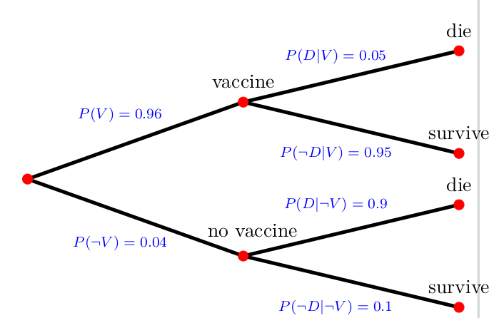
You read on Facebook that in the year 2021 about over 80% of people that died were vaccinated. You are shocked by this high probability that a dead person was vaccinated, \(P(V|D)\). You decide to check this fact. Reading the study to which the Facebook post is referring, you find out that the study only refers to people above the age of 90. Moreover, you find the following Tree Diargram. It allows checking the fact as it describes the vaccination rates and the conditional probabilities of people to die given the fact they were vaccinated or not. In particular, \(D\) denotes the event of die and \(\neg D\) denotes not die, i.e., survive; \(V\) denotes the event of vaccinated and \(\neg V\) not vaccinated.
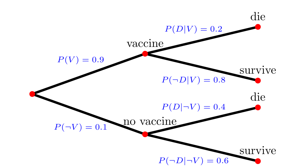
Figure 3.14: Tree: To die or not to die
- Calculate the overall probability to die, \(P(D)\)
- Calculate the probability that a person that has died was vaccinated, \(P(V|D)\).
- Your calculations shows that the fact used in the statement on Facebook is indeed true. Discuss whether this number should have an impact to get vaccinated or not.
Disclaimer: The case presented here is fictitious. The data given here are purely fictitious and serve only to practice the method.
Please find solution to the exercise in the appendix.
Exercise 3.11 Corona false positive
Suppose that Corona infects one out of every 1000 people in a population and that the test for it comes back positive in 99% of all cases if a person has Corona. Moreover, the test also produces some false positive, that is about 2% of uninfected patients also tested positive.
Now, assume you are tested positive and you want to know the chances of having the disease. Then, we have two events to work with:
A: you have Corona
B: your test indicates that you have Corona
and we know that \[\begin{align*} P(A)&=.001 \qquad \rightarrow \text{one out of 1000 has Corona}\\ P(B|A)&=.99 \qquad \rightarrow \text{probability of a positive test, given infection}\\ P(B|\neg A)&=.02 \qquad \rightarrow \text{probability of a false positive, given no infection} \end{align*}\]
As you don`t like to go into quarantine, you are interested in the probability of having the disease given a positive test, that is \(P(A|B)\)?
Disclaimer: The case presented here is fictitious. The data given here are purely fictitious and serve only to practice the method.
Please find solution to the exercise in the appendix.
3.5 Cognitive biases in decision making
In section 2.7, we discussed how human beings have limited cognitive abilities to arrive at optimal solutions. Behavioral economics, pioneered by Amos Tversky (1937-1996) and 2002 Nobel Prize winner Daniel Kahnemann (*1934), has identified several biases that explain why and when people fail to act perfectly rationally. In the following sections, we will explore some of the most prominent biases that arise from humans relying on heuristics in decision-making. Specifically, we will describe biases result from the use of availability, representative, and confirmation heuristics and can lead to flawed decision-making and negative outcomes for individuals and organizations. By recognizing and accounting for these biases, we can make better decisions.
3.5.1 Availability heuristic
The availability heuristic refers to our tendency to make judgments or decisions based on information that is easily retrievable from memory. For example, if someone hears a lot of news about a particular stock or investment, they may be more likely to invest in it, even if there are other better investment options available. This bias can also lead individuals to overestimate the frequency of certain events, such as the likelihood of a market crash, based on recent media coverage.
3.5.2 Representative heuristic
The representative heuristic refers to our tendency to make judgments based on how similar something is to a stereotype or preconceived notion. For example, an investor might assume that a company with a flashy website and marketing materials is more successful than a company with a more low-key image, even if the latter is actually more profitable. This bias can also lead to assumptions about the performance of certain investment strategies based on their resemblance to other successful strategies.
3.5.3 Confirmation heuristic
The confirmation heuristic refers to our tendency to seek out information that confirms our existing beliefs and ignore information that contradicts them. For example, an investor who strongly believes in the potential of a particular investment might only read news and analysis that supports their belief and ignore any information that suggests otherwise. This can lead to a failure to consider potential risks and downsides of an investment.
Exercise 3.12 Twelve cognitive biases
In the textbook of Bazerman & Moore (2012) twelve cognitive biases that are described. Read chapter 2 of the book and summarize the twelve biases in a sentence.
Please find solution to the exercise in the appendix.
3.6 Decision making and money
3.6.1 Financial literacy
You are financially literate if you understand and manage personal finances effectively. It involves having a basic understanding of financial concepts, such as budgeting, saving, investing, and managing debt. Financial literacy also includes knowledge of financial products and services, such as bank accounts, credit cards, loans, and insurance. Being financially literate means having the skills and knowledge to make informed financial decisions, and being able to assess risks and opportunities when it comes to managing money. It is an important life skill that can help individuals achieve their financial goals, build wealth, and avoid financial pitfalls.
Being better-educated was always associated with having more financial knowledge (Figure 1) across the countries we examined,3 yet we also found that education is not enough. That is, even well-educated people are not necessarily savvy about money.
Unfortunately, financial illiteracy is widespread. While being better-educated is associated with making better financial decisions on average, “even well-educated people are not necessarily savvy about money” (Mitchell & Lusardi, 2015, p. 3).
There are various attempts to assess the levels of financial literacy. See https://www.oecd.org/finance/financial-education/measuringfinancialliteracy.htm for example.
Exercise 3.13 S&P Global FinLit Survey
One example of a comprehend way to measure financial literacy stems from the Standard & Poor`s Ratings Services Global Financial Literacy Survey (see Klapper & Lusardi, 2020). They ask the following multiple-choice questions:
- Suppose you have some money. Is it safer to put your money into one business or investment, or to put your money into multiple businesses or investments?
- One business or investment
- Multiple businesses or investments
- Don`t know
- Refused to answer
- Suppose over the next 10 years the prices of the things you buy double. If your income also doubles, will you be able to buy less than you can buy today, the same as you can buy today, or more than you can buy today?
- Less
- The same
- More
- Don`t know
- Refused to answer
- Suppose you need to borrow $100. Which is the lower amount to pay back: $105 or $100 plus 3%?
- $105
- $100 plus 3%
- Don`t know
- Refused to answer
- Suppose you put money in the bank for 2 years and the bank agrees to add 15% per year to your account. Will the bank add more money to your account the second year than it did the first year, or will it add the same amount of money both years?
- More
- The same
- Don`t know
- Refused to answer
- Suppose you had $100 in a savings account and the bank adds 10% per year to the account. How much money would you have in the account after 5 years if you did not remove any money from the account?
- More than $150
- Exactly $150
- Less than $150
- Don`t know
- Refused to answer
These questions cover four fields of financial literacy, i.e., risk diversification, inflation and purchasing power, numeracy (simple calculations related to interest rates), and compound interest (interest payments increase exponentially over time). Knowledge in these concepts is important to make good financial decisions and to manage risk.
Try to answer these quesions and compare your performance with the results shown in Klapper & Lusardi (2020).
Please find solution to the exercise in the appendix.
Exercise 3.14 The big three questions
Referring to Mitchell & Lusardi (2015), only 21.7% of individuals in Germany with a lower secondary education and 72% of those with tertiary education can correctly answer all three of the following questions. Try it yourself!
- Suppose you had $100 in a savings account and the interest rate was 2% per year. After 5 years, how much do you think you would have in the account if you left the money to grow?
- More than $102
- Exactly $102
- Less than $102
- Do not know
- Refuse to answer
- Imagine that the interest rate on your savings account was 1% per year and inflation was 2% per year. After 1 year, how much would you be able to buy with the money in this account?
- More than today
- Exactly the same
- Less than today
- Do not know
- Refuse to answer
- Please tell me whether this statement is true or false: “Buying a single company’s stock usually provides a safer return than a stock mutual fund.”
- True
- False
- Do not know
- Refuse to answer
These three questions are designed to measure Lusardi & Mitchell (2014) reports that in many countries the financial illiteracy is considerably high as the following table shows:
| % all correct | % none correct | |
|---|---|---|
| Germany | 57 | 10 |
| Netherlands | 46 | 11 |
| United States | 35 | 10 |
| Italy | 28 | 20 |
| Sweden | 27 | 11 |
| Japan | 27 | 17 |
| New Zealand | 27 | 4 |
| Russia | 3 | 28 |
Please find solution to the exercise in the appendix.
3.6.2 Common investment mistakes
Investing can be a daunting task, but avoiding some common investment mistakes can help set you on the right path to financial success. The following list list shows according to Stammers (2016) the Top 20 common investment mistakes without the explanations provided in the paper:
- Expecting too much or using someone else’s expectations
- Not having clear investment goals
- Failing to diversify enough
- Focusing on the wrong kind of performance
- Buying high and selling low
- Trading too much and too often
- Paying too much in fees and commissions
- Focusing too much on taxes
- Not reviewing investments regularly
- Taking too much, too little, or the wrong risk
- Not knowing the true performance of your investments
- Reacting to the media
- Chasing yield
- Trying to be a market timing genius
- Not doing due diligence
- Working with the wrong adviser
- Letting emotions get in the way
- Forgetting about inflation
- Neglecting to start or continue
- Not controlling what you can
Exercise 3.15 Common investment mistakes
Read the paper and summarize the 20 mistakes.
Please find solution to the exercise in the appendix.
3.6.3 Simple financial mathematics
I discuss financial mathematics in the following chapter just briefly. If you want to gather a deeper understanding, I recommend the open textbook of Dahlquist et al. (2022) or the respective chapters of Wilkinson (2022).
3.6.3.1 Simple Interest
Suppose \(r\) denotes annual interest rates, \(P\) denotes the initial deposit which earns the interest, \(A\) denotes the value of the deposit at the end of an investment. Then, the relationship of these for a single year is
\[ A=P+Pr=P(1+r) \]
and for many years, \(t\), it is
\[ A=P(1+rt) \]
which is the simple interest formula. It gives the amount due when the annual interests does not become part of the deposit \(P\).
3.6.3.2 Compound interest
If the annual interest, \(P(1+r)\), is added to \(P\), we need a formula that takes this into account, and for two periods this is
\[ A=P\cdot [(1+r)\cdot(1+r)]=P(1+r)^2 \]
and for t periods
\[ A=P(1+r)^t. \]
Compound interest is the addition of interest to the principal sum of a loan or deposit, or in other words, interest on principal plus interest. It is the result of reinvesting interest, or adding it to the loaned capital rather than paying it out, or requiring payment from borrower, so that interest in the next period is then earned on the principal sum plus previously accumulated interest.
\[ A=P\left(1+\frac{r}{n}\right)^{nt} \]
Example
Suppose a principal amount of $1,500 is deposited in a bank paying an annual interest rate of 4.3%, compounded quarterly. Then the balance after 6 years is found by using the formula above, with \(P = 1500\), \(r = 0.043\) (4.3%), \(n = 4\), and \(t = 6\):
\[ A=1500\times\left(1+\frac{0.043}{4}\right)^{4\times 6}\approx 1938.84 \]
So the amount \(A\) after 6 years is approximately $1,938.84.
Subtracting the original principal from this amount gives the amount of interest received: \(1938.84-1500=438.84\)
3.6.3.3 Continuously compounded interest
As \(n\), the number of compounding periods per year, increases without limit, the case is known as continuous compounding, in which case the effective annual rate approaches an upper limit of \(e^r- 1\), where \(e\) is a mathematical constant that is the base of the natural logarithm.
Continuous compounding can be thought of as making the compounding period infinitesimally small, achieved by taking the limit as \(n\) goes to infinity. The amount after \(t\) periods of continuous compounding can be expressed in terms of the initial amount \(P\) as
\[ A=Pe^{rt} \]
3.6.3.4 Present value
The present is the value of an expected income stream determined as of the date of valuation. The present value is usually less than the future value because money has interest-earning potential, a characteristic referred to as the time value of money, except during times of zero- or negative interest rates, when the present value will be equal or more than the future value. Time value can be described with the simplified phrase, ``A dollar today is worth more than a dollar tomorrow’‘. Here, ’worth more’ means that its value is greater than tomorrow. A dollar today is worth more than a dollar tomorrow because the dollar can be invested and earn a day’s worth of interest, making the total accumulate to a value more than a dollar by tomorrow.
\[ P=Ae^{-rt} \]
3.6.4 Net present value and internal rate of return
When making decisions about financial products such as investments or loans, it is important to consider their long-term impact on your finances. Net Present Value (NPV) and Internal Rate of Return (IRR) are two key indicators that can help guide decision making and determine whether a financial product is a good investment.
Net Present Value (NPV) is the difference between the present value of all cash inflows and the present value of all cash outflows over a given time period. The formula to calculate NPV is:
\[ NPV = \sum_{n=1}^{N} \frac{C_n}{(1+r)^n} - C_0 \]
where \(C_n\) denotes net cash inflow during the period \(n\), \(r\) the discount rate, or the cost of capital, \(n\) the number of periods, and \(C_0\) the initial investment.
In other words, NPV helps determine the current value of future cash flows, adjusted for the time value of money. A positive NPV indicates that an investment is expected to generate a return greater than the cost of capital, while a negative NPV suggests that the investment is likely to result in a loss.
Internal Rate of Return (IRR), on the other hand, is the discount rate that makes the NPV of all cash inflows equal to the NPV of all cash outflows. The formula to calculate IRR is:
\[ 0 = \sum_{n=0}^{N} \frac{C_n}{(1+IRR)^n} \]
where \(C_n\) denotes the net cash inflow during the period \(n\), \(IRR\) the internal rate of return, \(n\) the number of periods, and \(C_0\) the initial investment.
IRR can be thought of as the rate of return an investment generates over time, taking into account the time value of money. When comparing different investment opportunities, a higher IRR generally indicates a more profitable investment.
Both NPV and IRR are important tools to help individuals make informed decisions about financial products. By comparing the NPV and IRR of different investment options, individuals can determine which investments are likely to generate the greatest returns over time, and which products may not be worth the initial investment.
It is worth noting that while NPV and IRR are useful indicators for decision making, they are not the only factors to consider. Individuals should also consider other important factors such as risk, liquidity, and diversification when evaluating different financial products. By taking a holistic approach and considering all relevant factors, individuals can make informed decisions that are best suited to their financial goals and circumstances.
Exercise 3.16 Investment case
You deposit 1,000 euros today into a savings account with an annual interest rate of 5% for 2 years. What is the balance after 2 years with annual, semi-annual (4 interest payments per year), and continuous compounding?
Please find solution to the exercise in the appendix.
Exercise 3.17 Present value
You want to have 100,000 in 10 years, and you can save money with an interest rate of 5% p.a. How much do you need to invest today for annual, semi-annual (4 interest periods), and continuous compounding to achieve your goal?
Please find solution to the exercise in the appendix.
Exercise 3.18 Invest in A or B
You are considering investing in project A or B.
Project A: It costs 50,000 today and is expected to generate cash flows of 20,000 per year for the next 5 years. You have a required rate of return of 8%.
Project B: It costs 50,000 today and you get 100,000 back in 5 years.
Calculate the value of your invest after five years. Which investment is the better one?
Please find solution to the exercise in the appendix.
Exercise 3.19 Net present value
You are considering investing in project A or B.
Project A: It costs 50,000 today and is expected to generate cash flows of 20,000 per year for the next 5 years. You have a required rate of return of 8%.
Project B: It costs 50,000 today and you get 100,000 back in 5 years.
Calculate the net present value of both projects and decide where to invest.
Please find solution to the exercise in the appendix.
Exercise 3.20 Internal rate of return
You are considering investing in project A or B.
Project A: It costs 50,000 today and is expected to generate cash flows of 20,000 per year for the next 5 years. You have a required rate of return of 8%.
Project B: It costs 50,000 today and you get 100,000 back in 5 years.
Calculate the internal rate of return of both projects with the help of a software package such as Excel or Libre Calc and decide where to invest.
Please find solution to the exercise in the appendix.
Exercise 3.21 Rule of 70
The Rule of 70 is often used to approximate the time required for a growing series to double. To understand this rule calculate how many periods it takes to double your money when it growth at a constant rate of 1% each period.
Please find solution to the exercise in the appendix.
3.6.5 A note on growth rates and the logarithm
Most data are recorded for discrete periods of time (e.g., quarters, years). Consequently, it is often useful to model economic dynamics in discrete periods of time. A good linear approximation to a growth rate from time \(t=0\) to \(t=1\) in \(x\) is \(\ln x_0 - \ln x_1\):
\[ \frac{x_1 - x_0}{x_0} \approx \ln x_1 - \ln x_0 \]
Let us prove that with some numbers of per capita real GDP for the US and Japan in 1950 and 1989:
What are the annual average growth rates over this period for the US and Japan? Here is one way to answer this question:
\[ Y_{1989} = (1 + g)^{39} \cdot Y_{1950} \]
Consequently, \(g\) can be calculated as:
\[ (1 + g) = \left(\frac{Y_{1989}}{Y_{1950}}\right)^{\frac{1}{39}} \]
Yielding \(g = 0.0195\) for the US and \(g = 0.0597\) for Japan. The US grew at an average growth rate of about 2% annually over the period, while Japan grew at about 6% annually.
The following method gives a close approximation to the answer above and will be useful in other contexts. A useful approximation is that for any small number \(x\): \(\ln (1 + x) \approx x\)
Now, we can take the natural log of both sides of:
\[ \frac{Y_{1989}}{Y_{1950}} = (1 + g)^{39} \]
to get:
\[ \ln (Y_{1989}) - \ln (Y_{1950}) = 39 \cdot \ln (1 + g) \]
which rearranges to:
\[ \ln (1 + g) = \frac{\ln (Y_{1989}) - \ln (Y_{1950})}{39} \]
and using our approximation:
\[ g \approx \frac{\ln (Y_{1989}) - \ln (Y_{1950})}{39} \]
In other words, log growth rates are good approximations for percentage growth rates. Calculating log growth rates for the data above, we get \(g \approx 0.0194\) for the US and \(g \approx 0.0582\) for Japan. The approximation is close for both.
Plotting growth using the logarithm
Recall that, with a constant growth rate \(g\) and starting from time 0, output in time \(t\) is:
\[Y_t = (1 + g)^t \cdot Y_0\]
Taking natural logs of both sides, we have:
\[\ln Y_t = \ln Y_0 + t \cdot \ln (1 + g)\]
We see that log output is linear in time. Thus, if the growth rate is constant, a plot of log output against time will yield a straight line. Consequently, plotting log output against time is a quick way to eyeball whether growth rates have changed over time.
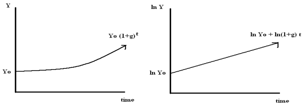
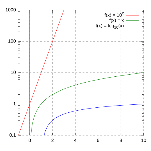
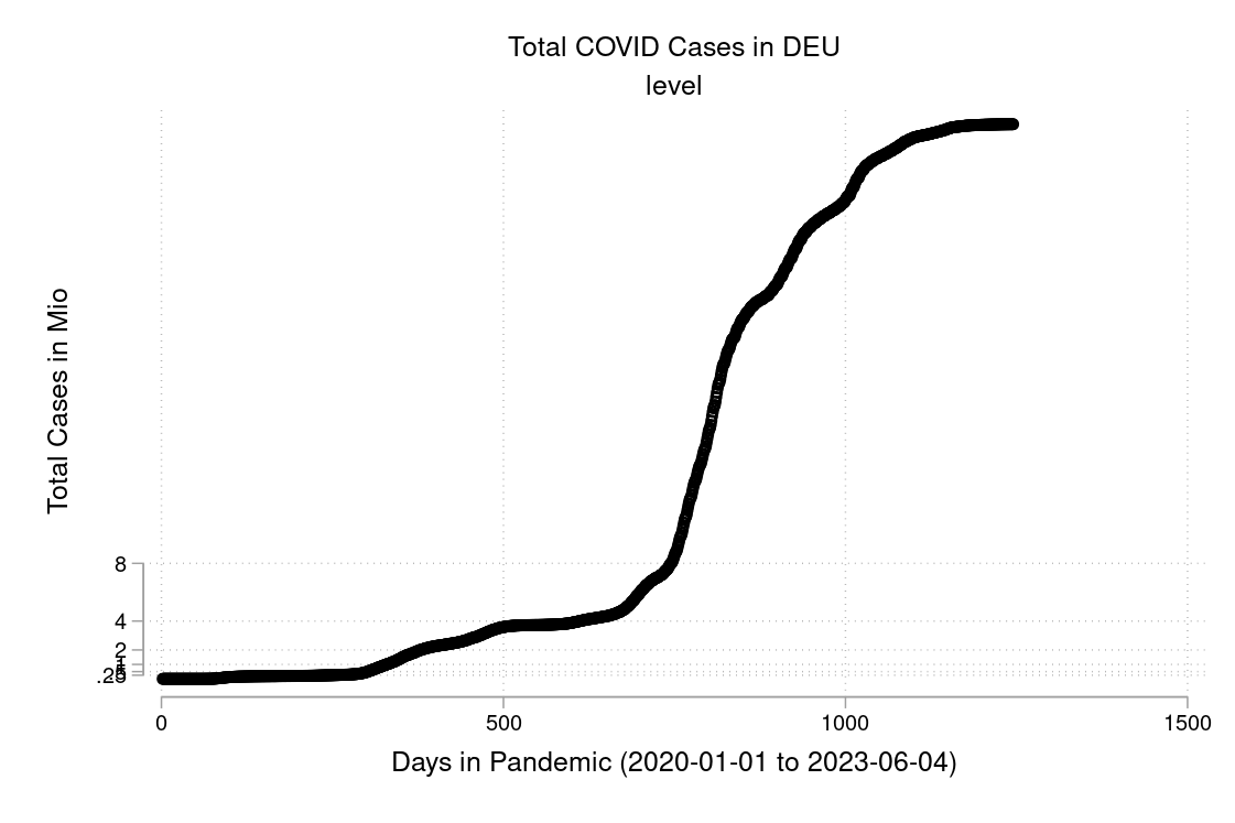
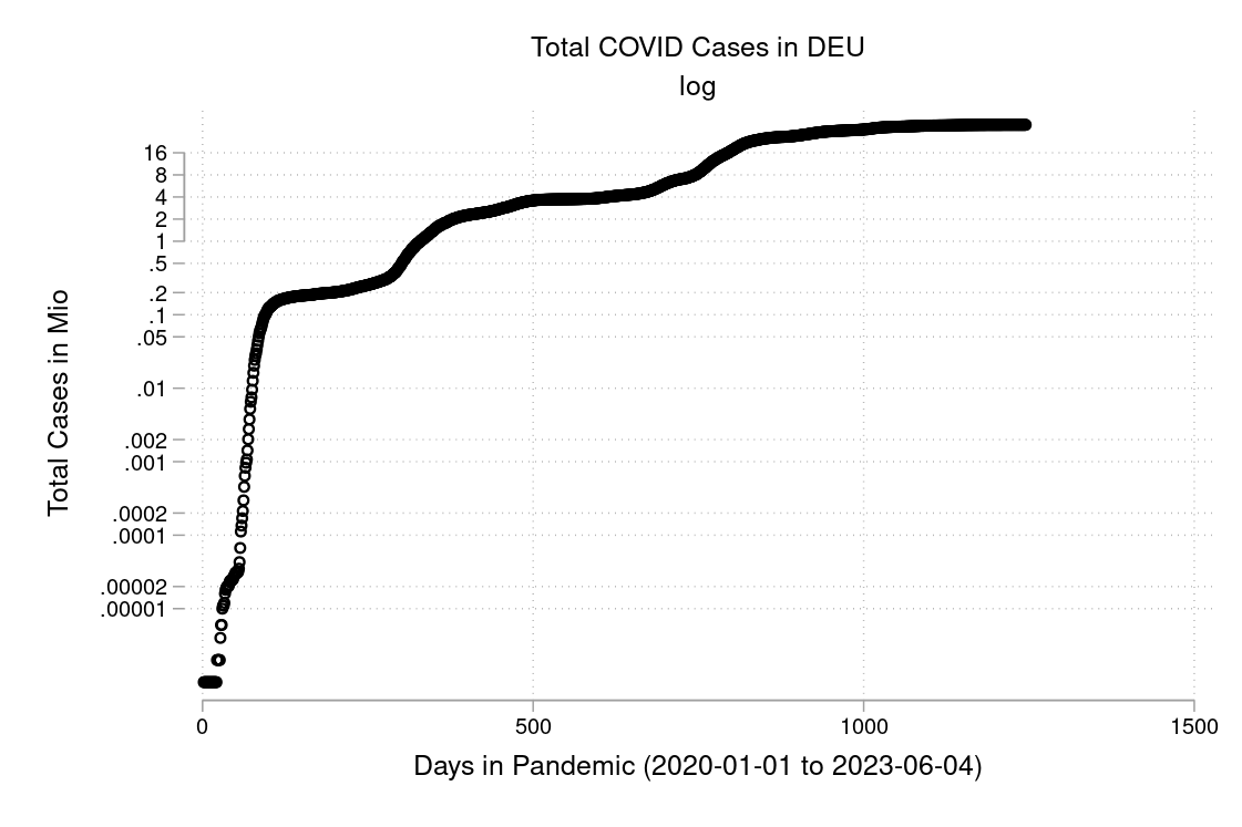
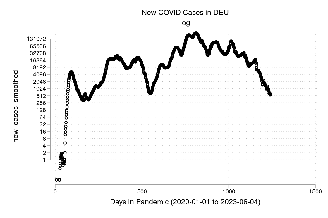
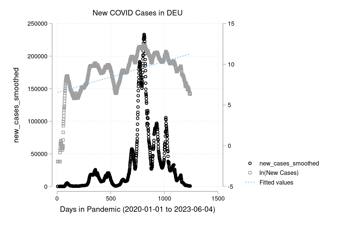
In figure 3.15 and 3.16 you see a semi-logarithmic plot that has one axis on a logarithmic scale and the other on a linear scale. It is useful for data with exponential relationships, where one variable covers a large range of values, or to zoom in and visualize that what seems to be a straight line in the beginning is, in fact, the slow start of a logarithmic curve that is about to spike, and changes are much bigger than thought initially.
Exercise 3.22 Investments over time Describe the formulas to describe the growth process of an investment over time when time is discrete and when time is continuous.
Please find solution to the exercise in the appendix.
Exercise 3.23 Exponential growth
Sketch a timeline for each of the following series:
- \(a_t=a_{t-1}+g\)
- \(\ln(a_t)\)
- \(b_t=b_{t-1}\cdot (1+g)\)
- \(\ln b_t\)
Please find solution to the exercise in the appendix.
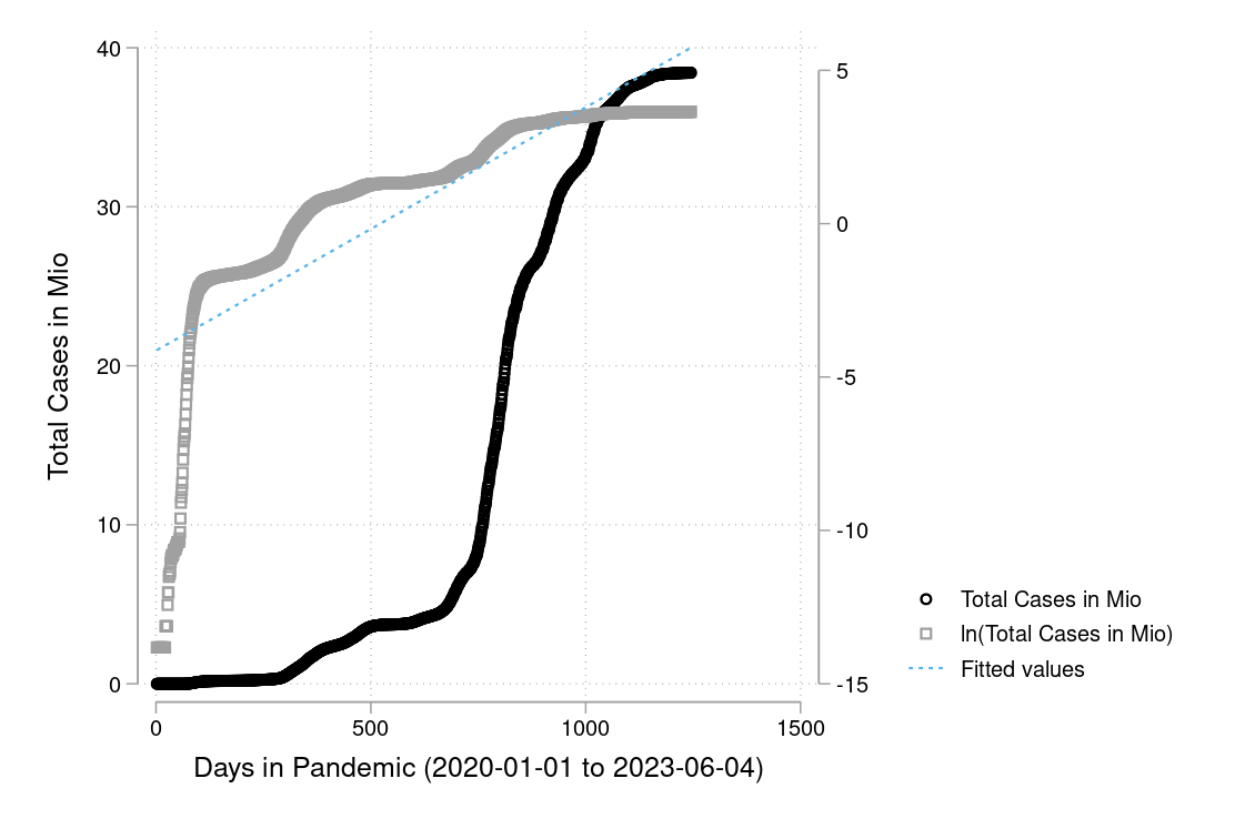
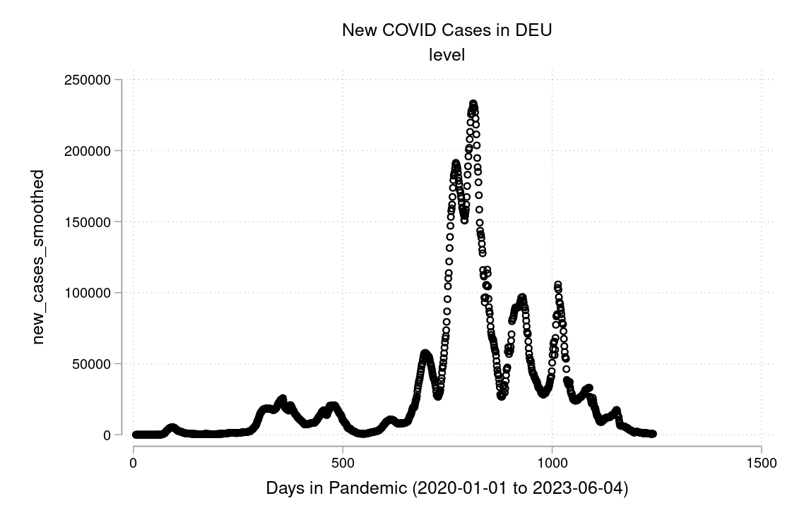
Exercise 3.24 COVID and how to plot it
I downloaded the complete Our World in Data COVID-19 dataset from ourworldindata.org. I created some graphs which I will show you below. Can you discuss the scaling and how to interpret them? What is your opinion on these graphs? Are some of them a bit misleading (at least if you don’t look twice)?
The example is taken from Morse et al. (2014, p. 134f).↩︎
Picture is taken from http://www-history.mcs.st-and.ac.uk/history/PictDisplay/Lagrange.html↩︎
This is a snapshot of a YouTube clip, see: https://youtu.be/8mjcnxGMwFo↩︎
Also see: http://www.sfu.ca/~wainwrig/5701/notes-lagrange.pdf↩︎