4 Managerial microeconomics
4.1 Consumption and production choices
In microeconomics, utility maximization (in its simplest form when having just two goods) involves selecting a combination of two goods that satisfies two essential conditions, see figure 4.1:
- The chosen point of utility maximization must fall within the attainable region defined by the Production Possibility Frontier (PPF) or be affordable within the constraints of a given budget.
- The selected point of utility maximization must lie on the highest indifference curve that is consistent with the first condition.
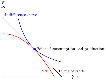
These conditions ensure that the consumer selects the optimal bundle of goods that maximizes their utility while taking into account the constraints imposed by production capabilities or budget limitations.
By analyzing production possibilities and individual preferences, economists gain insights into how consumers make choices, allocate resources, and achieve utility maximization. Understanding these concepts helps economists explore the trade-offs and decision-making processes that influence consumer behavior and shape market dynamics.
If you are not familiar with the basic principles of the production possibility frontier curve, indifference curves, and budget constraints, I recommend referring to section 6.1 of the appendix for a comprehensive overview. This section provides a detailed explanation and exploration of these concepts.
4.1.1 The role of income and budget
If income increases the budget constraint curve shifts outwards (to the right) as shown in figure 4.2.
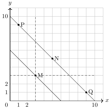
The utility-maximizing choice on the original budget constraint is M. The dashed horizontal and vertical lines extending through point M allow you to see at a glance whether the quantity consumed of goods on the new budget constraint is higher or lower than on the original budget constraint. On the new budget constraint, a choice like N will be made if both goods are normal goods. If good \(x\) is an inferior good, a choice like P will be made. If good \(y\) is an inferior good, a choice like Q will be made.
4.1.2 The role of prices
If price of one good increases then the budget constraint curve. When the price rises, the budget constraint shifts in to the left for that good.
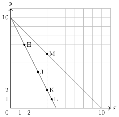
The dashed lines make it possible to see at a glance whether the new consumption choice involves less of both goods, or less of one good and more of the other. The new possible choices would be good \(x\)’s and more good \(y\)’s, like point H, or less of both goods, as at point J. Choice K would mean that the higher price of good \(x\) led to exactly the same quantity of good \(x\) being consumed, but fewer of good \(y\). Choices like L are theoretically possible (if good \(x\) are giffen goods) but highly unlikely in the real world, because they would mean that a higher price for goods \(x\) means a greater quantity consumed of good \(x\).
4.1.3 Substitution and income effect
When prices increase, individuals typically respond by reducing their consumption of the product with the higher price. This reaction is driven by two factors, both of which can occur simultaneously.
The substitution effect occurs when a price change incentivizes consumers to consume less of a good with a relatively higher price and more of a good with a relatively lower price.
The income effect stems from the fact that a higher price effectively reduces the purchasing power of income (even if actual income remains the same). This reduction in purchasing power leads to a decrease in the consumption of the good, particularly when the good is considered normal.
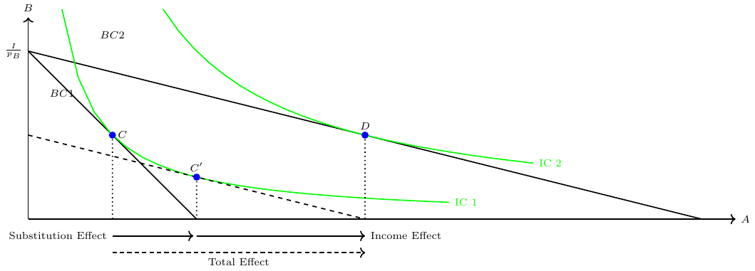
Figure 4.4 illustrates the Hicksian decomposition for a price reduction of good \(A\), which affects the consumption of goods \(A\) and \(B\), shifting the consumption point from \(C\) to \(D\). The point \(C'\) represents the hypothetical consumption point resulting from a rotated budget constraint that reflects the new price relationship.
Exercise 4.1 The graphical foundations of demand curves
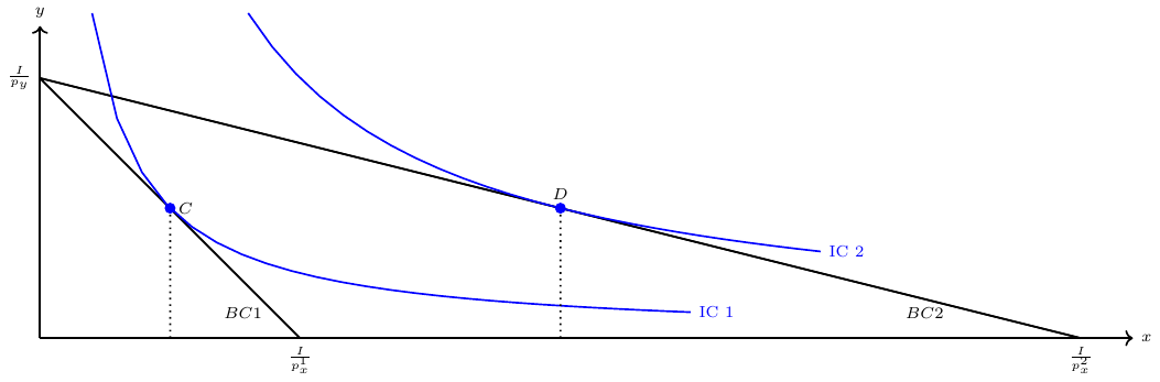
A shift in the budget constraint means that when individuals are seeking their highest utility, the quantity that is demanded of that good will change. In this way, the logical foundations of demand curves—which show a connection between prices and quantity demanded—are based on the underlying idea of individuals seeking utility.
In Figure 4.5, two points of consumption are displayed, illustrating the optimal choices made by customers when faced with prices \(p_x^1>p_x^2\). The objective of this exercise is to graphically derive the demand function for good \(x\). To accomplish this, please provide a second two-dimensional plot below the existing graph, with the price of good \(x\), \(p_x\), represented on the y-axis.
Exercise 4.2 Derivation of demand function using the Lagranian multiplier
A representative consumer has on average the following utility function: \(U=x y,\) and faces a budget constraint of \(B=P_{x} x+P_{y} y,\) where \(B, P_{x}\) and \(P_{y}\) are the budget and prices, which are given. Solve the following choice problem:
Maximize \(U=x y\) s.t. \(B=P_{x} x+P_{y} y\).
Please find solution to the exercise in the appendix.
Exercise 4.3 Cobb-Douglas and demand
A consumer who has a Cobb-Douglas utility function \(u(x, y)=A x^{\alpha} y^{\beta}\) faces the budget constraint \(p x+q y=I\), where \(A, \alpha, \beta, p,\) and \(q\) are positive constants. Solve the problem:
\[ \begin{array}{lll} \max A x^{\alpha} y^{\beta} & \text { subject to } & p x+q y=I \end{array} \]
Please find solution to the exercise in the appendix.
4.1.4 Consumption, production, and terms of trade
Market prices in a closed economy: The price relation of two goods, the so-called terms of trade, is determined by the slope of the Production Possibility Frontier (PPF) at the point where it is tangent to the indifference curve. This relationship highlights the trade-off between the two goods and their relative scarcity within a closed economy.
Utility maximizing production: The production point that maximizes utility is where the PPF is tangent to the price relation, i.e. the terms of trade. This principle applies not only in a closed economy (autarky) but also under free trade (open economy). It implies that producers should allocate resources in a way that balances the trade-off between producing more of one good at the expense of another, while considering consumer preferences. Figure 4.1 depicts this.
Exercise 4.4 Understanding indifference curves and budget constraints
- Which indifference curve in the figure on the right represents the highest utility level? Explain your decision.
- Suppose two goods are perfect substitutes. Draw the indifference curves for perfect substitutes.
- Suppose two goods are perfect complements. Draw the indifference curves for perfect complements.
- Suppose you have a fixed income \(I=10\) that you can spend on consuming two goods \(x, y\) at certain prices \(p_x=1, p_y=1\). Draw the budget line consisting of all possible combinations of two goods that a consumer can buy at certain market prices by allocating his income. Using indifference curves, sketch what each consumer should consume to maximize utility.
Please find solution to the exercise in the appendix.
Exercise 4.5 Utility maximization
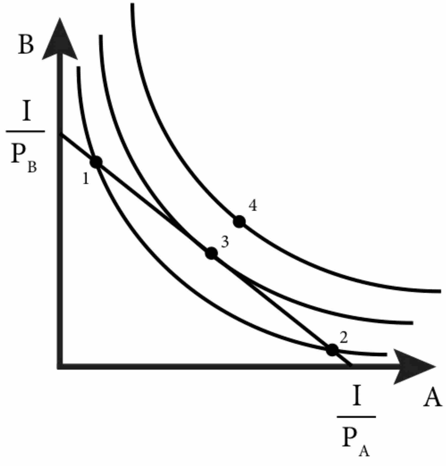
Figure 4.6 stems from Emerson (2019, ch. 4). Use the following sentences to describe the respective points in the figure.
- Optimal bundle.
- Can do better by trading some B for some A.
- Can do better by trading some B for some A.
- Unaffordable.
Please find solutions to the exercise in Emerson (2019, ch. 4).
4.2 Markets under perfect competition
Perfect competition is never found in the real world. However, it is a useful theoretical model that serves as a reference point for analyzing real-world markets. It provides valuable insights into market functioning and informs policymakers on how to address instances of market failure, where at least one assumption of perfect markets is not met.
The assumptions of perfect markets and perfect competition, respectively, are:
Many buyers and sellers: In a perfectly competitive market, there are numerous buyers and sellers, none of whom have a significant influence over market price. Each participant is a price taker, meaning they have no control over the price at which goods or services are exchanged.
Homogeneous products: The products offered by all firms in a perfectly competitive market are identical or homogeneous. Consumers perceive no differences between the goods or services provided by different sellers. As a result, buyers base their purchase decisions solely on price.
Perfect information: All buyers and sellers in a perfectly competitive market have complete and accurate information about prices, quality, availability, and other relevant factors. This assumption ensures that market participants can make rational decisions and respond efficiently to changes in market conditions.
Free entry and exit: Firms can freely enter or exit the market in response to profits or losses. There are no barriers to entry or exit, such as legal restrictions or substantial costs, that prevent new firms from entering the market or existing firms from leaving it.
Perfect mobility of factors of production: The resources used in production, such as labor and capital, can move freely between different firms and industries. There are no constraints on the mobility of factors of production, allowing firms to allocate resources efficiently.
Profit maximization: All firms in a perfectly competitive market are profit maximizers. They aim to maximize their profits by adjusting their output levels based on prevailing market conditions. If firms can increase their profits, they will expand production, and if they incur losses, they will reduce output or exit the market.
No externatlities: There are assumed to be no externalities, that is no external costs or benefits to third parties not involved in the transaction.
These assumptions collectively define perfect competition and form the foundation of its analysis. If all conditions are fulfilled, there is no need for government regulation. Welfare is maximized and no pareto-improvement can be achieved.
Theory would predict that if firms in an industry would make some profits, new firms will enter the market or existing firms would produce more which both yields an increase in supply. That, in turn, will drive down market prices until all firms earn zero profits and no more firms would have an incentive to enter the market. In the equilibrium, total revenue equals total cost. Thus, firms do not make profits. Firms can only make profits if they have some sort of competitive advantage and hence are not price takers which would be against assumption 1. The most extreme form of competitive advantage is a monopoly. It describes that one firm is the only provider of a certain good or service. This firm can set prices and the supply of the good and service completely. We will discuss that extreme case in the next section.
4.3 Monopoly
A monopolist is a firm that is the only provider of a good or service. There is no close substitute to it. The ability of a monopolist to raise its price above the competitive level by reducing output is known as market power. This implies a loss of total welfare. In contrast with a perfectly competitive firm which faces a perfectly elastic demand (taking price as given), a monopolist faces the market demand. As a consequence, a monopolist has the power to set the market price. While we can consider a competitive firm as a price taker, a monopolist is price decision-maker or price setter. Firms that have to face fierce competition are more like price takers as they cannot set the price above the market price. If firms in perfect competition would set the price higher, all consumers would simply stop buying from that particular firm. That is not the case for a firm with market power, that is, a firm that has a product with unique features no other competitor has to offer.
Revenue function
There are two types of constraints that restrict the behavior of a monopolist (and any other firm):
- Technological constraints summarized in the cost function \(C(x)\).
- Demand constraints: \(x(p)\).
Thus, we can write the revenue (or profit) function of the monopolist in two alternative ways:
Either by using the demand function: \[ \pi(p) = px(p) - C(x(p)) \]
Or by using the inverse demand function: \[ \pi(x) = p(x)x - C(x) \]
The demand, \(x(p)\), and the inverse demand, \(p(x)\), represent the same relationship between price and demanded quantity from different points of view. The demand function is a complete description of the demanded quantity at each price, whereas the inverse demand gives us the maximum price at which a given output \(x\) may be sold in the market.
Revenue and price relationship
Thus, an increase in production by a monopolist has two opposing effects on revenue:
- A quantity effect: one more unit is sold, increasing total revenue by the price at which the unit is sold.
- A price effect: in order to sell the last unit, the monopolist must cut the market price on all units sold. This decreases total revenue.
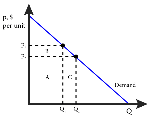
The two effects are shown in figure 4.7: At price \(p_1\), the total revenue is \(p_1 \cdot Q_1\), which is represented by the areas A+B. At price \(p_2\), the total revenue is \(p_2 \cdot Q_2\), which is represented by the areas A+C. Area A is the same for both, so the marginal revenue is the difference between B and C or C-B. Note that area C is the price, \(p_2\), times the change in quantity, \(Q_2 - Q_1\), or \(p \Delta Q\); and area B is the quantity, \(Q_1\), times the change in price, \(p_2 - p_1\), or \(\Delta p \cdot Q\). Since \(p_2 - p_1\) is negative, the change in total revenue is C-B or: \(\Delta TR = p \Delta Q + \Delta p \cdot Q\). Dividing both sides by \(\Delta Q\) gives us an expression for marginal revenue:
\[ MR = \frac{\Delta TR}{\Delta Q} = \underbrace{p}_{\text{quantity effect}} + \underbrace{Q \frac{\Delta p}{\Delta Q}}_{\text{price effect}} \]
Profit-maximizing level of output
To find the profit-maximizing price and quantity, respectively, we should look at the first-order conditions:
\[\begin{align*} \max_{p} \pi (p) \equiv& \max_{p} \quad px(p) - C(x(p))\\ \frac{\partial \pi (p)}{\partial p} =& \pi ' (p) = x(p) + px'(p) - C'(x(p))x'(p) \overset{!}{=} 0 \end{align*}\]
or
\[\begin{align*} \max_{p} \pi (x) \equiv& \max_{x} \quad p(x)x - C(x)\\ \frac{\partial \pi (x)}{\partial x} =& \pi ' (p) = \underbrace{p(x)}_{\text{quantity effect}} + \underbrace{xp'(x)}_{\text{price effect}} - C'(x) \overset{!}{=}& 0\\ \Rightarrow \underbrace{p(x) + xp'(x)}_{\text{marginal revenue}} =& \underbrace{C'(x)}_{\text{marginal costs}}\\ \Rightarrow MR =& MC \end{align*}\]
At the profit-maximizing level of output, marginal revenue equals marginal cost, that is, an infinitesimal change in the level of output changes revenue and cost equally. In other words, an infinitesimal increase in the level of output increases revenue and cost by the same amount, and an infinitesimal decrease in the level of output reduces revenue and cost by the same amount.
Thus, we can determine a monopoly firm’s profit-maximizing price and output by following three steps:
- Determine the demand, marginal revenue, and marginal cost curves.
- Select the output level at which the marginal revenue and marginal cost curves intersect.
- Determine from the demand curve the price at which that output can be sold.
Price effect of a monopoly
Due to the price effect of an increase in output, the marginal revenue curve of a firm with market power always lies below its demand curve. So, a profit-maximizing monopolist chooses the output level at which marginal cost is equal to marginal revenue—not equal to price. As a result, the monopolist produces less and sells its output at a higher price than a perfectly competitive industry would. It earns a profit in the short run and the long run.
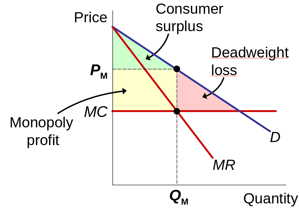
Welfare
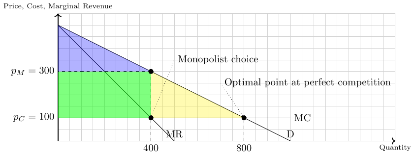
As illustrated in Figure 4.8, the price-setting behavior of a monopolist typically leads to a reduction in overall welfare: The shaded green area represents the monopoly profit, and the blue area denotes the consumer surplus, the sum of both constitute the total welfare. The yellow triangle represents the deadweight loss, indicating the welfare that is lost due to the monopolist producing fewer goods at a higher price than in a competitive market. The horizontal line at \(p=100\) represents the marginal costs (MC).
Price elasticity and market power
We know that the demand elasticity of price can be measured with:
\[ \frac{\triangle p/\bar{p}}{\triangle x / \bar{x}}. \]
Using differential calculus, the point-price elasticity of demand (PPD) can be written as:
\[ PPD = \frac{\partial p(x)}{\partial x} \cdot \frac{x}{p(x)} \]
This can also be expressed as:
\[ PPD = p'(x) \frac{x}{p(x)} = x \frac{p'(x)}{p(x)} \]
Thus, if \(PPD = 0\), the price does not change if a single firm increases its quantity sold on the market. That means the firms are price takers, and their quantity sold has no impact on the price. If firms, however, have market power, \(PPD < 0\), which means that if a firm increases the quantity on the market, the price must fall. The PPD can hence be interpreted as an indicator of the market power of firms.
Marginal revenue and price elasticity
Now, plugging the PPD into the MR function, we can show that MR is equal to zero when we have a unit demand elasticity, PPD, of \(-1\):
\[ MR = p(x) + xp'(x) = p(x)\left(1 + x\frac{p'(x)}{p(x)}\right) = p(x)\left(1 + PPD\right) \]
Also see figure 4.9. In the monopoly output, marginal revenue and marginal cost are equal:
\[ MC = p(x) \cdot \left(1 + PPD\right) \]
Lerner index
The Lerner index is a measure of monopoly power, which equals the markup over marginal cost as a percentage of price. To obtain the Lerner index of monopoly power (or market power), let us rearrange \(MC = p(x) \cdot \left(1 + PPD\right)\) as follows:
\[ \frac{MC - p(x)}{p(x)} = PPD = \text{Lerner Index} \]
If a firm does not have market power (\(PPD = 0\)), its price equals the marginal cost. When a firm’s market power is high (up to \(|PPD| = \infty\)), the higher the markup that a firm sets. In perfect competition, since \(p\) and MC are equal, the Lerner Index is 0. A pure monopolist, on the other hand, can theoretically charge an infinite markup, which leads us to a Lerner index of 1.
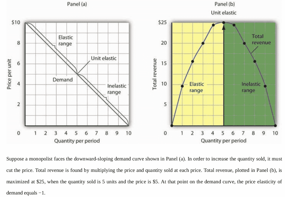
Exercise 4.6 Marginal revenue and total revenue
Show the relationship between a linear demand curve and the marginal revenue curve in one panel and the relationship of the quantity sold and the total revenue in another panel. What characterizes the price of a profit maximizing monopolist?
Please find solution to the exercise in the appendix.
Exercise 4.7 How to maximize profits
A company sold a quantity of 750 goods (\(Q_{t=1}=750\)) in January (\(t=1\)), at a price of 45 € (\(P_{t=1}=45\)). In February (\(t=2\)), they reduced the price to 40 Euro (\(P_{t=2}=40\)) and sold 800 goods (\(Q_{t=2}=800\)). Now answer the following questions knowing that the total costs had been 26,500 € in January and 28,000 € in February.
- Calculate the price elasticity of demand at the current prices.
- Derive the demand function.
- Derive the cost function.
- Derive the revenue function.
- Derive the marginal revenue function.
- Derive the marginal cost function.
- Calculate the profit-maximizing price and output.
- Calculate the amount of profit in January, February, and what the company can expect by setting the prices profit-maximizing.
Please find solution to the exercise in the appendix.
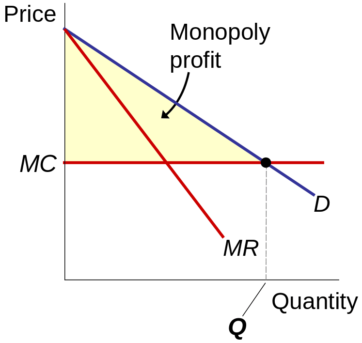
4.3.1 Monopoly and price discrimination
Discrimination is the practice of treating people differently based on some (irrelevant) characteristic, such as race or gender. It is important to actively fight discrimination whenever it is observed. However, the concept of discrimination takes a different form when it comes to price discrimination, which is a business practice involving the sale of the same goods at different prices to different buyers. This practice can be commonly seen in special offers tailored for students or retired individuals.
One of the key factors utilized in price discrimination is the willingness to pay (WTP) of individuals. By charging a higher price to buyers with a higher WTP, a firm can maximize its profit. Moreover, and that is kind of surprising, it also comes with a increase in social welfare as is shown in figure 4.11 and figure 4.11. In 4.11, the monopolist charges the same price (PM) to all buyers. A deadweight loss results. In 4.11, however, the monopolist produces the competitive quantity but charges each buyer his or her WTP. This is called perfect price discrimination. The monopolist captures all consumer surplus as profit. But there is no deadweight loss.
In the real world, price discrimination is a common phenomenon, but achieving perfect price discrimination is highly challenging. This is primarily because no firm possesses complete knowledge of every buyer’s willingness to pay (WTP), and buyers typically do not disclose this information to sellers. Consequently, firms often divide customers into groups based on observables that are likely correlated with their WTP.
4.4 Regional Economics
4.4.1 Von Thünen model of land use
The classical model of spatial organization of the economy stems Heinrich von Thünen (1783-1850). The model focuses on agriculture as this was the dominant use of land at the time. However, the fundamental ideas of the model can be applied to various industries. The model can be described as follows: Assume a focal point of demand for agricultural goods (e.g., the marketplace of a large city). Differences in soil quality in the agricultural periphery of the considered city are neglected. The demand is differentiated. That means, various goods such as grains, dairy products, meat, timber, vegetables are required to satisfy the needs of the people. The goods differ in terms of
- the market price they can achieve,
- the assumed constant marginal production costs \((c_i)\),
- the revenue per unit of land, and
- in terms of their transportability, that is, each good has different specific transport costs \((\theta_i)\).
All mentioned variables are exogenously given. In particular, the model is based on the following assumptions:
- Point-centered demand for all goods \(i\).
- Different production methods possible, each with constant (marginal) production costs \(c_i\).
- Homogeneous Space: The agricultural land surrounding the central marketplace is assumed to be uniform and homogeneous in terms of soil fertility, climate, and other relevant factors.
- Given market prices for the individual products \(p_i\)
- Producers supply the market and have linear product-specific transportation costs \((\theta_i)\).
- Perfect competition: The model assumes perfect competition among farmers for the available land (free market access). That implies that they have full knowledge of market conditions and make rational decisions.
To analyze the model, let us start by considering the restriction to a single land use. The key idea is that the rent price for a unit of land arises from the net yield that this unit of land enables under that particular land use. However, since both production costs and distance-dependent transport costs need to be subtracted from the gross yield to determine the net yield, it follows that land rent is determined by the distance from the center. Under a given land use, the value of an agricultural area is significantly influenced by its distance from the marketplace.
Formally, the land rent for land use for production of good \(i\), depending on the distance \(x\) from the marketplace, is given by:
\[ r_i(x) = q_i(p_i - c_i - \theta_i \cdot x) \]
The land rent increases with the quantity demanded \((q)\) and the price of the good, and it decreases with the marginal production costs \((c)\), the specific transportation costs \((\theta)\), and the distance \((x)\) from the marketplace. The typical shape of a rent curve, with \(r\) on the y-axis and \(x\) on the x-axis, is a linearly decreasing curve. Its slope is determined by the expression \(-q_i \theta_i\). Therefore, the steeper the specific transportation costs, the steeper the curve.
Suppose, different land uses are allowed. By varying the price, revenue, and cost parameters in the equation above, different rent curves with varying locations and slopes emerge for different land uses. The interesting question now is: How high will the market rent be?
Thünen provides a clear answer to this question: Competition among land tenants will ensure that in a specific distance zone around the center, the production method with the highest net yield in that zone will prevail. In other words, the market rent curve (or bid rent curve) is the upper envelope of all rent curves for specific production methods. The situation is illustrated in figure 4.12 and 4.13 for three different production methods. The intersections of the market rent curves determine the shifts in production zones.
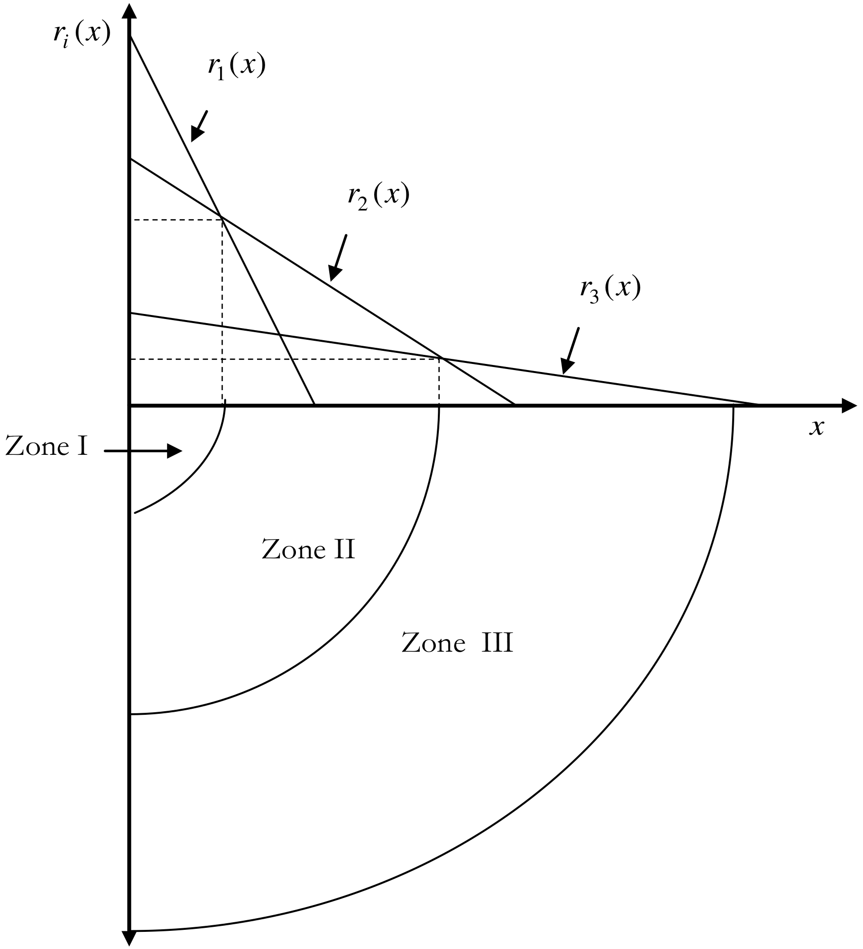
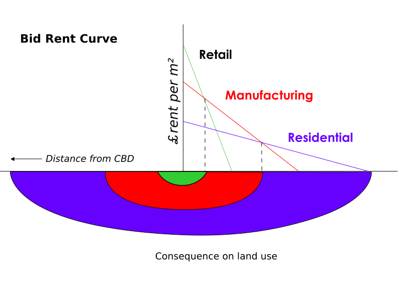
This model is also known as the Bid rent theory. A short but nice explanation of the model can be found on Wikipedia, see here.
Exercise 4.8 Agricultural land use
In the vicinity of an agglomeration center, four different agricultural land use forms are possible. We have information about the specific yield per unit of land \(q_i\), the (constant) marginal costs \(c_i\), the specific transportation costs \(\theta_i\), and the price \(p_i\) that can be achieved for a unit of the respective product in the center.
Where do we see which land use form?
| Production Form | Production Form | Production Form | Production Form | |
|---|---|---|---|---|
| \(i\) | 1 | 2 | 3 | 4 |
| \(q_i\) | 10 | 5 | 30 | 20 |
| \(p_i\) | 5 | 5 | 2 | 6 |
| \(c_i\) | 1 | 2 | 1 | 5 |
| \(\theta_i\) | 0.4 | 0.1 | 0.15 | 0.05 |
Exercise 4.9 Business location model
The Thünenian approach is intended to be applied to a business location model. The customer frequency, depending on the distance \(x\) from the center, can be approximated by the following function:
\[ f(x)_i = A_{0} e^{-a x} \]
The probability of sale per square meter for business type \(i\) is denoted by \(\lambda_i\). The business types also differ in terms of profit margin and fixed costs. Describe the market rent curve and show which business type will dominate in each location. What effects does an increase in the parameter \(a\) have? What about an increase in \(A_0\)? Interpret the changes in parameters and the results from an economic perspective.
4.4.2 Launhardt/Hotelling location model
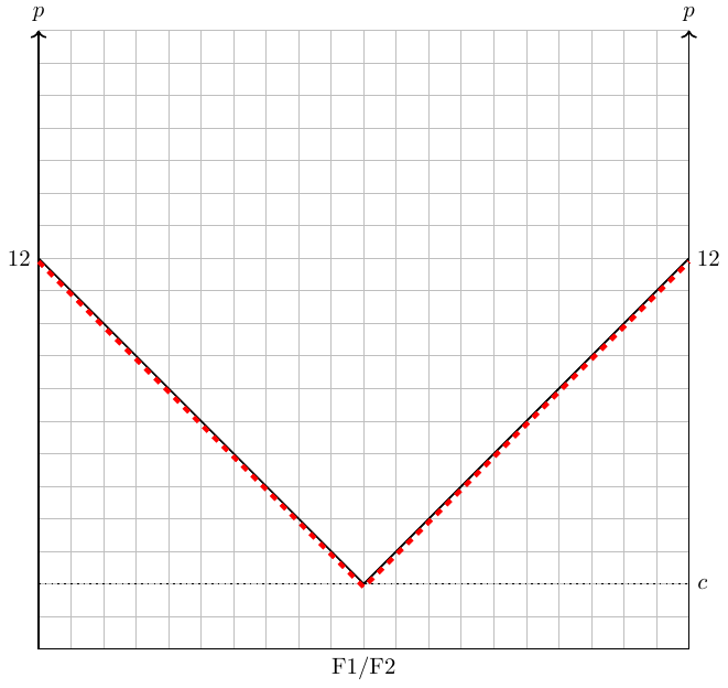
Consider a scenario where two firms, i.e., \(i={F1;F2}\), have the option to establish their locations along a linear market, such as a street or a beach. These firms can relocate without incurring any costs and sell an identical product at the same price. Consequently, the only means of competition available to them is by strategically selecting their respective locations. Moreover, assume that customers are uniformly distributed throughout the market, and each customer is willing to purchase one unit of the product up to a certain price, denoted as \(\bar{p}\). The cost of transportation is the same for both firms and is proportional to the distance between the firm and the customer.
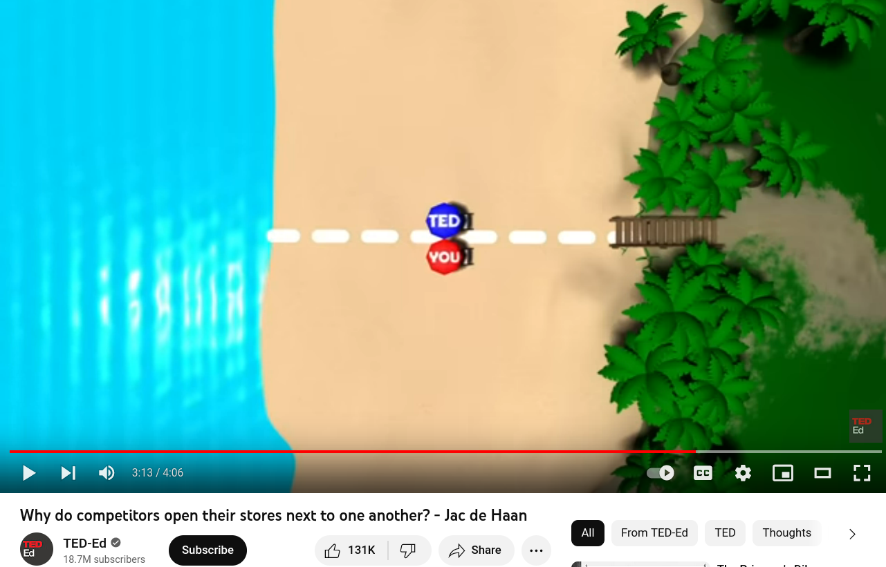
If we assume that the transportation costs are equal for both firms and that the market has a finite size, the firms will eventually position themselves at the center of the market with no empty space between them. The rationale and dynamics behind this behavior are clearly explained in the YouTube clip of TED-Ed Why do competitors open their stores next to one another? - Jac de Haan, see figure 4.14. I highly recommend watching the clip.
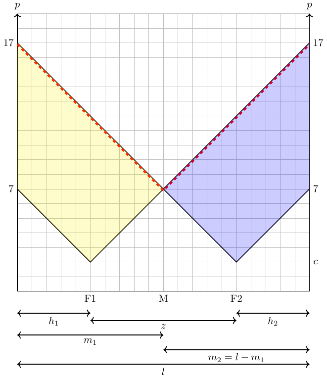
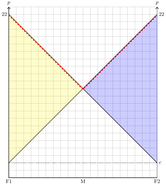
If we assume that the transportation costs can vary between the two firms, things became a bit more complicated. Let us define transportation costs for a firm as \(\theta_i=a_i d(x)\), where \(d(x)\) represents the distance between the company and the respective costumer and \(a_i\) is firm-specific costs of transportation. Let us further assume competition and loosen the assumption of fixed prices: Firms can set prices but they need to charge the price of the good, \(p\), plus their costs of transporting the good to the costumer. Thus, the price of a good a firm needs to charge in order not to make deficits is \[ p^{min}(x)=c+\theta_i=c+a_i d(x) \]
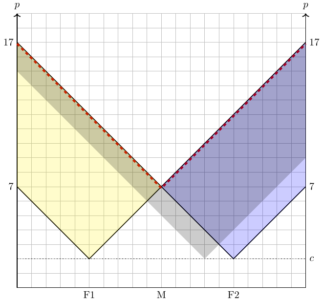
If we assume that the transport costs are the same for both firms and that the market is limited in size, the firms will end up at the center of the market with no space inbetween them. However, there is always an incentive to deviate from that minimum of spatial differentiation. However, the dynamic is kind of strange as we can show in the following four figures.
Graph stems from Anon (2020, p. 344)↩︎
The graph stems from https://en.wikipedia.org/wiki/File:Bid_rent1.png↩︎
Taken from https://youtu.be/jILgxeNBK_8↩︎