8 Regression analysis
8.1 Simple linear regression
The linear regression analysis is a widely used technique for predictive modeling. Its purpose is to establish a mathematical equation that relates a continuous response variable, denoted as \(y\), to one or more independent variables, represented by \(x\). The objective is to create a regression model that enables the prediction of the value of \(y\) based on known values of \(x\).
To ensure meaningful predictions, it is important to have an adequate number of observations, denoted as \(i\), available for the variables of interest.
The linear regression model can be expressed as: \[ y_i = \beta_{0} + \beta_{1} x_i + \epsilon_i, \] where the index \(i\) denotes the individual observations, ranging from \(i = 1\) to \(n\). The variable \(y_i\) represents the dependent variable, also known as the regressand. The variable \(x_i\) represents the independent variable, also referred to as the regressor. \(\beta_0\) denotes the intercept of the population regression line, a.k.a. the constant. \(\beta_1\) denotes the slope of the population regression line. Lastly, \(\epsilon_i\) refers to the error term or the residual, which accounts for the deviation between the predicted and observed values of \(y_i\).
By fitting a linear regression model, one aims to estimate the values of \(\beta_0\) and \(\beta_1\) in order to obtain an equation that best captures the relationship between \(y\) and \(x\).
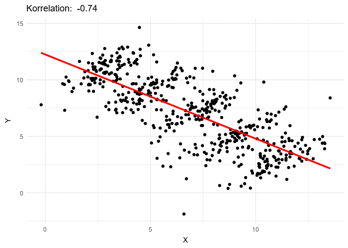
While the correlation coefficient and the slope in simple linear regression are similar in many ways, it’s important to note that they are not identical. The correlation coefficient measures the strength and direction of the linear relationship between variables in a broader sense, while the slope in simple linear regression specifically quantifies the change in the dependent variable associated with a unit change in the independent variable.
8.1.1 Estimating the coefficients of the linear regression model
In practice, the intercept and slope of the regression are unknown. Therefore, we must employ data to estimate the unknown parameters, \(\beta_0\) and \(\beta_1\). The method we use is called the ordinary least squared (OLS) method. The idea is to minimize the sum of the squared differences of all \(y_i\) and \(y_i^*\) as sketched in Figure 8.1.
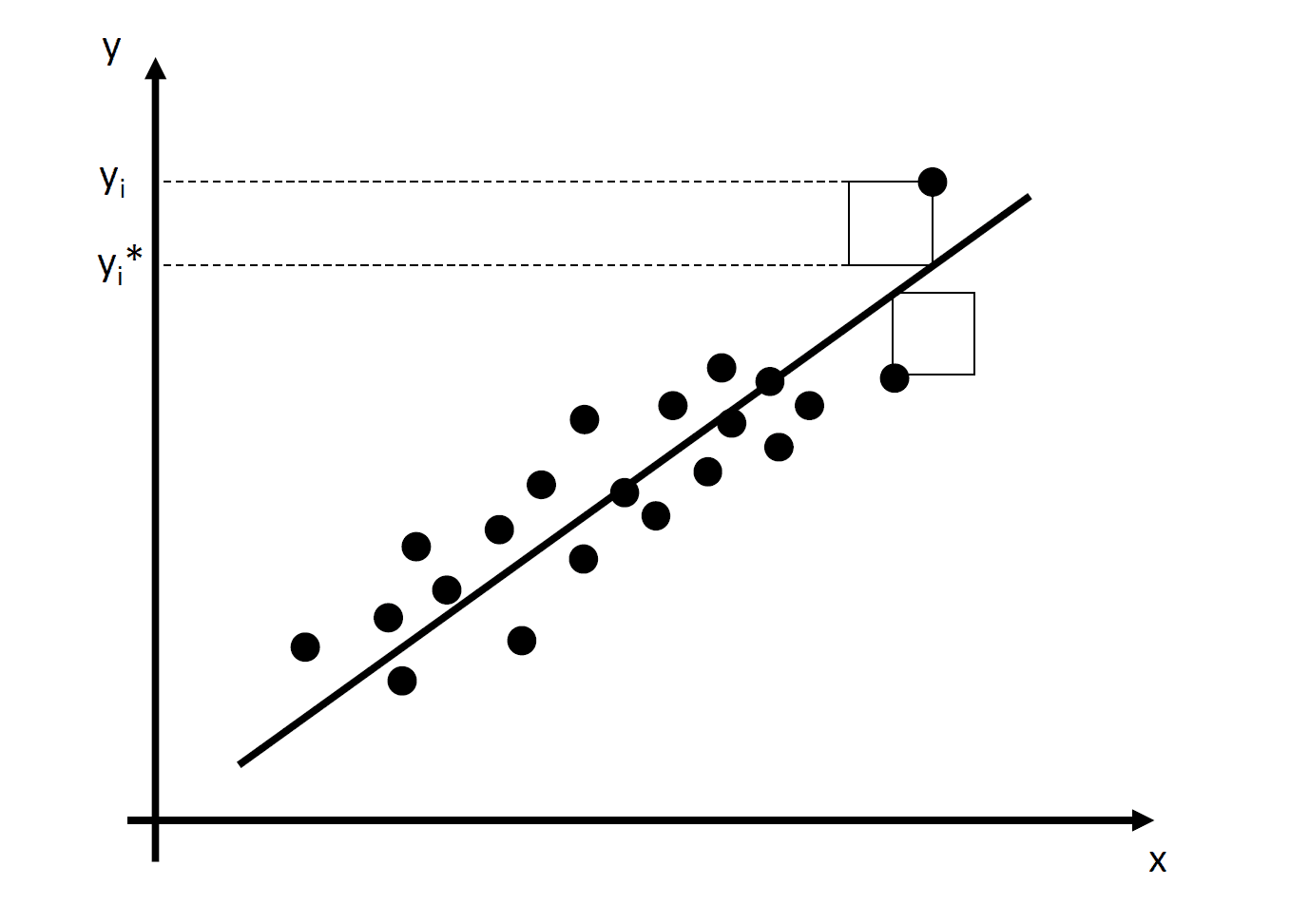
Thus, we minimize the squared residuals by choosing the estimated coefficients \(\hat{\beta_{0}}\) and \(\hat{\beta_{1}}\) \[\begin{align*} \min_{\hat{\beta_{0}}, \hat{\beta_{1}}}\sum_{i=1} \epsilon_i^2 &= \sum_{i=1} \left[y_i - \underbrace{(\hat{\beta_{0}} + \hat{\beta_{1}} x_i)}_{\textnormal{predicted values}\equiv y_i^*}\right]^2\\ \Leftrightarrow &= \sum_{i=1} (y_i - \hat{\beta_{0}} - \hat{\beta_{1}} x_i)^2 \end{align*}\] Minimizing the function requires to calculate the first order conditions with respect to alpha and beta and set them zero: \[\begin{align*} \frac{\partial \sum_{i=1} \epsilon_i^2}{\partial \beta_{0}}=2 \sum_{i=1} (y_i - \hat{\beta_{0}} - \hat{\beta_{1}} x_i)=0\\ \frac{\partial \sum_{i=1} \epsilon_i^2}{\partial \beta_{1}}=2 \sum_{i=1} (y_i - \hat{\beta_{0}} - \hat{\beta_{1}} x_i)x_i=0 \end{align*}\] This is just a linear system of two equations with two unknowns \(\beta_{0}\) and \(\beta_{1}\), which we can mathematically solve for \(\beta_0\): \[\begin{align*} &\sum_{i=1} (y_i - \hat{\beta_{0}} - \hat{\beta_{1}} x_i)=0\\ \Leftrightarrow \hat{\beta_{0}}&=\frac{1}{n}\sum_{i=1} (y_i - \hat{\beta_{1}} x_i)\\ \Leftrightarrow \hat{\beta_{0}}&=\bar{y}-\hat{\beta_{1}}\bar{x} \end{align*}\] and for \(\beta_{1}\): \[\begin{align*} &\sum_{i=1} (y_i - \hat{\beta_{0}} - \hat{\beta_{1}} x_i)x_i=0\\ \Leftrightarrow & \sum_{i=1} y_i x_i- \underbrace{\hat{\beta_{0}}}_{\bar{y}-\hat{\beta_{1}}\bar{x}}x_i - \hat{\beta_{1}} x_i^2=0\\ \Leftrightarrow & \sum_{i=1} y_i x_i- (\bar{y}-\hat{\beta_{1}}\bar{x})x_i - \hat{\beta_{1}} x_i^2=0\\ \Leftrightarrow & \sum_{i=1} y_i x_i- \bar{y}x_i-\hat{\beta_{1}}\bar{x}x_i - \hat{\beta_{1}} x_i^2=0\\ \Leftrightarrow & \sum_{i=1} (y_i - \bar{y}-\hat{\beta_{1}}\bar{x} - \hat{\beta_{1}} x_i)x_i=0\\ % \Leftrightarrow & \sum_{i=1} (y_i - \bar{y})-\beta_{1}\bar{x} - \hat{\beta_{1}} x_i=0\\ \Leftrightarrow & \sum_{i=1} (y_i - \bar{y}) x_i -\hat{\beta_{1}}(\bar{x} - x_i)x_i =0\\ \Leftrightarrow & \sum_{i=1} (y_i - \bar{y}) x_i = \hat{\beta_{1}} \sum_{i=1} (\bar{x} - x_i) x_i \\ % \Leftrightarrow & \beta_{1} =\frac{\sum_{i=1}(y_i - \bar{y})x_i }{ \sum_{i=1} (\bar{x} - x_i)x_i }\\ \Leftrightarrow & \hat{\beta_{1}} =\frac{\sum_{i=1}(y_i - \bar{y})x_i }{ \sum_{i=1} (\bar{x} - x_i)x_i }\\ \Leftrightarrow & \hat{\beta_{1}} =\frac{\sum_{i=1}(y_i -\bar{y})(x_i-\bar{x})}{\sum_{i=1} (\bar{x} - x_i)^2 }\\ \Leftrightarrow & \hat{\beta_{1}} ={\frac {\sigma_{x,y}}{\sigma^2_{x}}} \end{align*}\] The estimated regression coefficient \(\hat{\beta_{1}}\) equals the covariance between \(y\) and \(x\) divided by the variance of \(x\).
The formulas presented above may not be very intuitive at first glance. The online version of the book Hanck et al. (2020) offers a nice interactive application in the box The OLS Estimator, Predicted Values, and Residuals that helps to understand the mechanics of OLS. You can add observations by clicking into the coordinate system where the data are represented by points. Once two or more observations are available, the application computes a regression line using OLS and some statistics which are displayed in the right panel. The results are updated as you add further observations to the left panel. A double-click resets the application, that means, all data are removed.
Hanck, C., Arnold, M., Gerber, A., & Schmelzer, M. (2020). Introduction to econometrics with R. University of Duisburg-Essen. www.econometrics-with-r.org
8.1.2 The least squares assumptions
OLS performs well under a quite broad variety of different circumstances. However, there are some assumptions which need to be satisfied in order to ensure that the estimates are normally distributed in large samples.
The Least Squares Assumptions should fulfill the following assumptions: \[ Y_i = \beta_0 + \beta_1 X_i + \epsilon_i \text{, } i = 1,\dots,n \]
- The error term \(\epsilon_i\) has conditional mean zero given \(X_i: E(u_i|X_i)=0\).
- \((X_i,Y_i), i=1,\dots,n\) are independent and identically distributed (i.i.d.) draws from their joint distribution.
- Large outliers are unlikely: \(X_i\) and \(Y_i\) have nonzero finite fourth moments. That means, assumption 3 requires that \(X\) and \(Y\) have a finite kurtosis.
8.1.3 Measures of fit
After fitting a linear regression model, a natural question is how well the model describes the data. Visually, this amounts to assessing whether the observations are tightly clustered around the regression line. Both the coefficient of determination and the standard error of the regression measure how well the OLS Regression line fits the data.
\(R^2\) is the fraction of the sample variance of \(Y_i\) that is explained by \(X_i\). Mathematically, the \(R^2\) can be written as the ratio of the explained sum of squares to the total sum of squares. The explained sum of squares (ESS) is the sum of squared deviations of the predicted values \(\hat{Y_i}\), from the average of the \(Y_i\). The total sum of squares (TSS) is the sum of squared deviations of the \(Y_i\) from their average. Thus we have \[\begin{align} ESS & = \sum_{i = 1}^n \left( \hat{Y_i} - \overline{Y} \right)^2, \\ TSS & = \sum_{i = 1}^n \left( Y_i - \overline{Y} \right)^2, \\ R^2 & = \frac{ESS}{TSS}. \end{align}\] Since \(TSS = ESS + SSR\) we can also write \[ R^2 = 1- \frac{\textcolor{blue}{SSR}}{\textcolor{red}{TSS}} \] with \[ SSR= \sum_{i = 1}^n \epsilon^2. \]
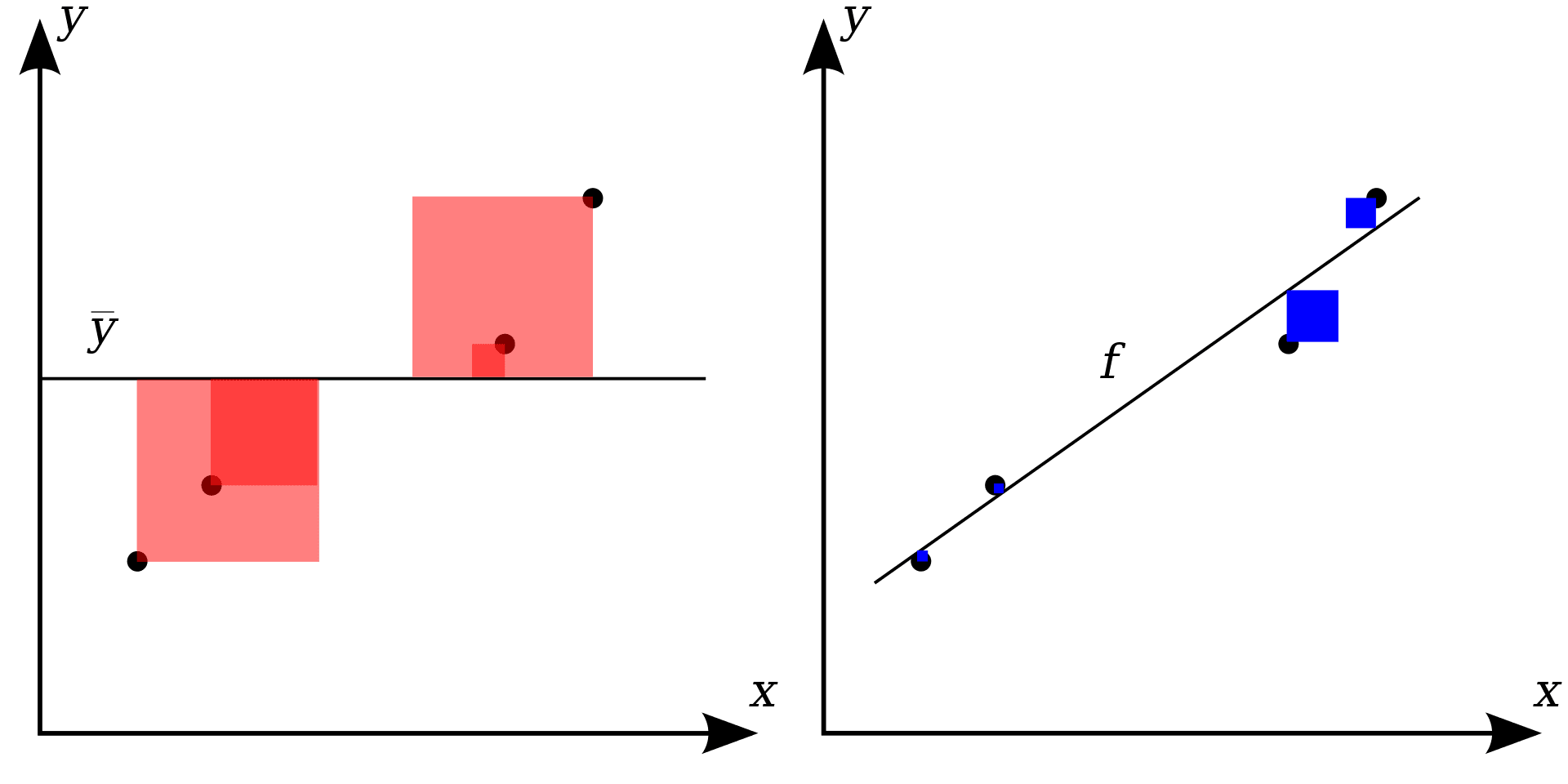
\(R^2\) lies between 0 and 1. It is easy to see that a perfect fit, i.e., no errors made when fitting the regression line, implies \(R2=1\) since then we have \(SSR=0\). On the contrary, if our estimated regression line does not explain any variation in the \(Y_i\), we have \(ESS=0\) and consequently \(R^2=0\). Figure 8.2 represents the relationship of TTS and SSR.
8.2 Multiple linear regression
Having understood the simple linear regression model, it is important to broaden our scope beyond the relationship between just two variables: the dependent variable and a single regressor. Our goal is to causally interpret the measured association of two variables, which requires certain conditions as explained in ?sec-identification.
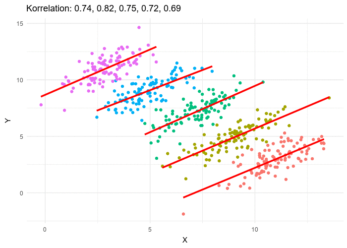
8.2.1 Simpson’s paradox and regressions
To illustrate this concept, let’s revisit the phenomenon known as Simpson’s paradox. Simpson’s paradox occurs when the overall association between two categorical variables differs from the association observed when we consider the influence of one or more other variables, known as controlling variables. This paradox highlights three key points:
It challenges the assumption that statistical relationships are fixed and unchanging, showing that the relationship between two variables can vary depending on the set of variables being controlled.
Simpson’s paradox is part of a larger class of association paradoxes, indicating that similar situations can arise in various contexts.
It serves as a reminder of the potential pitfalls of making causal inferences in nonexperimental studies, emphasizing the importance of considering confounding variables.
Thus, it is important to consider confounding variables to ensure valid and reliable causal interpretations in research, particularly in nonexperimental settings.
The multiple regression model can be expressed as:
\[ Y_i = \beta_0 + \beta_1 X_{1i} + \beta_2 X_{2i} + \beta_3 X_{3i} + \dots + \beta_k X_{ki} + u_i, \ i=1,\dots,n. \]
To estimate the coefficients of the multiple regression model, we seek to minimize the sum of squared mistakes by choosing estimated coefficients \(\beta_0,\beta_1,\dots,\beta_k\) such that:
\[ \sum_{i=1}^n (Y_i - b_0 - b_1 X_{1i} - b_2 X_{2i} - \dots - b_k X_{ki})^2 \]
This demands matrix notation which goes beyond the scope of this introduction.
8.2.2 Gauss-Markov and the best linear unbiased estimator
The Gauss-Markov assumptions, also known as the classical linear regression assumptions, are a set of assumptions that underlie the ordinary least squares (OLS) method for estimating the parameters in a linear regression model. These assumptions ensure that the OLS estimators are unbiased, efficient, and have desirable statistical properties.
The Gauss-Markov assumptions are as follows:
Linearity: The relationship between the dependent variable and the independent variables is linear in the population model. This means that the true relationship between the variables can be represented by a linear equation.
Independence: The errors (residuals) in the regression model are independent of each other. This assumption ensures that the errors for one observation do not depend on or influence the errors for other observations.
Strict exogeneity: The errors have a mean of zero conditional on all the independent variables. In other words, the expected value of the errors is not systematically related to any of the independent variables.
No perfect multicollinearity: The independent variables are not perfectly correlated with each other. Perfect multicollinearity occurs when one independent variable is a perfect linear combination of other independent variables, leading to problems in estimating the regression coefficients.
Homoscedasticity: The errors have constant variance (homoscedasticity) across all levels of the independent variables. This assumption implies that the spread or dispersion of the errors is the same for all values of the independent variables.
No endogeneity: The errors are not correlated with any of the independent variables. Endogeneity occurs when there is a correlation between the errors and one or more of the independent variables, leading to biased and inefficient estimators.
No autocorrelation: The errors are not correlated with each other, meaning that there is no systematic pattern or relationship between the errors for different observations.
These assumptions collectively ensure that the OLS estimators are unbiased, efficient, and have minimum variance among all linear unbiased estimators. Violations of these assumptions can lead to biased and inefficient estimators, invalid hypothesis tests, and unreliable predictions. Therefore, it is important to check these assumptions when using the OLS method and consider alternative estimation techniques if the assumptions are violated.
8.3 How to identify statistically significant estimated coefficients in a regression analysis
8.3.1 P-values
When you perform regression analysis, the results are often presented in a table that includes p-values. Understanding these p-values is essential to determine whether the relationships between your variables are statistically significant.
The p-value tells us the probability that the coefficient (effect) we observe is due to random chance rather than a real relationship. Thus, it ranges theoretically from 0 to 1.
- Threshold for Significance
Commonly used thresholds (also called significance levels) are:- 0.05 (5% significance level)
- 0.01 (1% significance level)
- 0.001 (0.1% significance level)
- Decision Rule for a 5% significance level:
- P-Value \(<\) 0.05: The result is considered statistically significant. There is strong evidence that the coefficient (relationship) is not due to random chance.
- P-Value \(\geq\) 0.05: The result is not considered statistically significant. There is not enough evidence to say that the coefficient is different from zero (no relationship).
Here is an example of a stylized regression table:
| Variable | Coefficient | P-Value |
|---|---|---|
| Intercept | 2.5 | 0.0001 |
| Study Hours | 0.8 | 0.0005 |
| Sleep Hours | 0.1 | 0.0450 |
| TV Watching | -0.3 | 0.0600 |
How can we interpret the p-values:
Intercept (P-Value: 0.0001): The p-value is much less than 0.05, indicating the intercept is statistically significant. This means the starting value (when all other variables are zero) is not due to chance.
Study Hours (P-Value: 0.0005): The p-value is less than 0.05, so the coefficient for Study Hours is statistically significant. This means there is strong evidence that more study hours are associated with higher scores, and this relationship is unlikely to be due to chance.
Sleep Hours (P-Value: 0.0450): The p-value is slightly less than 0.05, indicating that the coefficient for Sleep Hours is statistically significant. There is some evidence that more sleep hours are associated with higher scores.
TV Watching (P-Value: 0.0600): The p-value is greater than 0.05, meaning the coefficient for TV Watching is not statistically significant. There isn’t strong enough evidence to conclude that TV Watching affects scores.
Summary:
- P-values help you determine the significance of your results.
- A p-value less than 0.05 typically indicates a significant result, meaning the variable likely has an effect.
- A p-value greater than 0.05 suggests the variable’s effect is not statistically significant, and any observed relationship might be due to chance.
8.3.2 t-values
Understanding t-values helps to determine whether the relationships between your variables are statistically significant.
The t-value measures how many standard deviations the estimated coefficient is away from zero. It helps us understand if the coefficient is significantly different from zero (no effect).
- Threshold for Significance:
- The significance of a t-value depends on the chosen significance level (e.g., 0.05) and the degrees of freedom in the regression model.
- In regression analysis, “degrees of freedom” refer to the number of independent values that can vary in the calculation of a statistic, typically calculated as the number of observations minus the number of estimated parameters (including the intercept). This concept helps adjust the precision of the estimates and the validity of the statistical tests used in the analysis.
- A common rule of thumb is that a t-value greater than approximately 2 (or less than -2) indicates statistical significance at the 0.05 level.
- A little bit more precise is the value 1.96. It is often called the “magic number” as it is crucial in statistics because it marks the cutoff for a 95% confidence interval in a standard normal distribution, meaning 95% of data lies within 1.96 standard deviations of the mean. This makes it a key threshold for determining statistical significance in hypothesis testing at the 5% significance level.
- Decision Rule:
- |t-Value| \(>\) 1.96: The result is considered statistically significant. There is strong evidence that the coefficient (relationship) is not zero.
- |t-Value| \(\geq\) 1.96: The result is not considered statistically significant. There is not enough evidence to say that the coefficient is different from zero (no relationship).
Here is an example of a stylized regression table:
| Variable | Coefficient | t-Value |
|---|---|---|
| Intercept | 2.5 | 5.0 |
| Study Hours | 0.8 | 4.0 |
| Sleep Hours | 0.1 | 1.89 |
| TV Watching | -0.3 | -2.1 |
How can we interpret the t-values:
Intercept (t-Value: 5.0): The t-value is much greater than 2, indicating the intercept is statistically significant. This means the starting value (when all other variables are zero) is not due to chance.
Study Hours (t-Value: 4.0): The t-value is greater than 2, so the coefficient for Study Hours is statistically significant. This means there is strong evidence that more study hours are associated with higher scores, and this relationship is unlikely to be due to chance.
Sleep Hours (t-Value: 1.89): The t-value is less than 2 in absolute values. This indicates that the coefficient for Sleep Hours may be statistically insignificant, suggesting no evidence that more sleep hours are associated with higher scores.
TV Watching (t-Value: -2.1): The t-value is -2.1, which is more than 2 in absolute values. This suggests that there might be some evidence that more TV watching is associated with lower scores.
Summary:
- t-values help you determine the significance of your estimated coefficients.
- A t-value greater than 2 (or less than -2) typically indicates a significant result, meaning the variable likely has an effect.
- A t-value between -2 and 2 suggests the variable’s effect is not statistically significant, and any observed relationship might be due to chance.
8.3.3 Standard error
Understanding the standard error also helps to assess regression estimates. It measures the average distance that the observed values fall from the regression line. It provides an estimate of the variability of the coefficient.
The standard error (SE) of a coefficient quantifies the precision of the coefficient estimate. Smaller standard errors indicate more precise estimates. However, the standard error itself does not allow to judge on an estimate. Therefore, we need the t-values which can be calculated using the estimate and the SE as follows:
\[ t_{\hat {\alpha }}={\frac {{\hat {\alpha }}-\alpha _{0}}{s.e. ({\hat{\alpha }})}} \left(=\frac{\text{estimated value - hypothesized value}}{\text{standard error of the estimator}}\right), \] where \(\hat{\alpha }\) denotes the estimator of parameter \(\alpha\) in some statistical model, \(s.e. ({\hat{\alpha }})\) denotes the standard error of the estimator, and \(\alpha _{0}\) is the hypothesized value. That means, in a typical regression analysis, we are interested in whether the estimated value is different to zero, \(\alpha _{0}=0\). Thus, we test
\[ t_{\hat{\alpha}} = \frac{\hat{\alpha}}{s.e.(\hat{\alpha})}. \]
Here is an example of stylized regression table might look like, including standard errors:
Example: Calculating t-values
| Variable | Coefficient | Standard error |
|---|---|---|
| Intercept | 2.5 | 0.5 |
| Study Hours | 0.8 | 0.2 |
| Party Hours | -0.5 | 0.05 |
| TV Watching | -0.3 | 0.15 |
Using Table 8.1 we can practice the formula:
Intercept: \[ t_{\text{Intercept}} = \frac{2.5}{0.5} = 5.0 \]
Study Hours: \[ t_{\text{Study Hours}} = \frac{0.8}{0.2} = 4.0 \]
Party Hours: \[ t_{\text{Party Hours}} = \frac{-0.5}{0.05} = -10.0 \]
TV Watching: \[ t_{\text{TV Watching}} = \frac{-0.3}{0.15} = -2.0 \]
Table 8.2 contains the respective t-values:
| Variable | Coefficient | Standard Error | t-Value |
|---|---|---|---|
| Intercept | 2.5 | 0.5 | 5.0 |
| Study Hours | 0.8 | 0.2 | 4.0 |
| Party Hours | -0.5 | 0.05 | -10.0 |
| TV Watching | -0.3 | 0.15 | -2.0 |
Explanation of the t-values:
- Intercept (t-value: 5.0): The t-value of 5.0 indicates that the intercept is highly significant.
- Study Hours (t-value: 4.0): The t-value of 4.0 suggests that the coefficient for Study Hours is statistically significant.
- Party Hours (t-value: -10.0): The t-value of -10.0 shows a highly significant negative effect of Party Hours on the dependent variable.
- TV Watching (t-value: -2.0): The t-value of -2.0 indicates that the coefficient for TV Watching is significant, but less so compared to the other variables.
8.4 Statistical control requires causal justification
Tip 8.1
Scientific research revolves around challenging our own views and findings. A good researcher does not merely present their results; instead, they engage in discussions about potential limitations and pitfalls to draw valid conclusions. Engaging in polemics goes against the essence of good research. We should not conceal potential weaknesses in our scientific strategy or empirical approach; rather, we should emphasize their existence. Even if this disappoints individuals seeking easy answers, it is crucial to acknowledge these limitations. The Catalogue of Bias is an excellent resource that provides insight into various potential pitfalls and challenges encountered during research, which may sometimes be difficult to completely rule out.
The following sections discuss the necessity of statistical control when confounding effects are present, to avoid omitted variable bias in regression analysis. Additionally, we examine the impact of controlling for too many variables on regression estimates.
8.4.1 Confounding variables
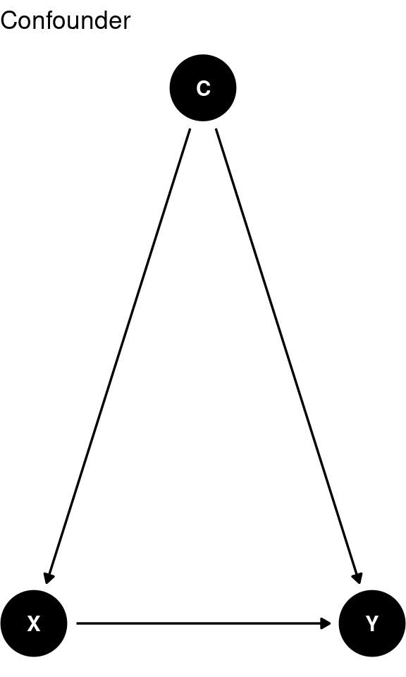
A confounding variable is a factor that was not accounted for or controlled in a study but has the potential to influence the results. In other words, the true effects of the treatment or intervention can be obscured or muddled by the presence of this variable.
For example, let’s consider a scenario where two groups of individuals are observed: one group took vitamin C daily, while the other group did not. Over the course of a year, the number of colds experienced by each group is recorded. It might be observed that the group taking vitamin C had fewer colds compared to the group that did not. However, it would be incorrect to conclude that vitamin C directly reduces the occurrence of colds. Since this study is observational and not a true experiment, numerous confounding variables are at play. One potential confounding variable could be the individuals’ level of health consciousness. Those who take vitamins regularly might also engage in other health-conscious behaviors, such as frequent handwashing, which could independently contribute to a lower risk of catching colds.
To address confounding variables, researchers employ control measures. The idea is to create conditions where confounding variables are minimized or eliminated. In the aforementioned example, researchers could pair individuals who have similar levels of health consciousness and randomly assign one person from each pair to take vitamin C daily (while the other person receives a placebo). Any differences observed in the number of colds between the groups would be more likely attributable to the vitamin C, compared to the original observational study. Well-designed experiments are crucial as they actively control for potential confounding variables.
Consider another scenario where a researcher claims that eating seaweed prolongs life. However, upon reading interviews with the study subjects, it becomes apparent that they were all over 80 years old, followed a very healthy diet, slept an average of 8 hours per day, drank ample water, and engaged in regular exercise. In this case, it is not possible to determine whether longevity was specifically caused by seaweed consumption due to the presence of numerous confounding variables. The healthy diet, sufficient sleep, hydration, and exercise could all independently contribute to longer life. These variables act as confounding factors.
A common error in research studies is to fail to control for confounding variables, leaving the results open to scrutiny. The best way to head off confounding variables is to do a well-designed experiment in a controlled setting. Observational studies are great for surveys and polls, but not for showing cause-and-effect relationships, because they don’t control for confounding variables.
Control variables are usually variables that you are not particularly interested in, but that are related to the dependent variable. You want to remove their effects from the equation. A control variable enters a regression in the same way as an independent variable – the method is the same.
Tip 8.2
Nick Huntington-Klein (2025) offers Causal Inference Animated Plots on his homepage. Read this online section and consider the animated graphs.
Huntington-Klein, N. (2025). Causal inference animated plots. online. https://www.nickchk.com/causalgraphs.html
8.4.2 Other controls
“Although it is possible to remove bias from an estimate of a causal path by controlling for a confounding variable, it is also easy to add bias to an estimate by controlling for a variable that is either not a confounder or does not block a confounding path” (Wysocki et al., 2022, p. 4)
The impact of statistical control varies depending on the type of control variable used. Cinelli et al. (2022) discuss various functional relationships and provides a comprehensive list of variables that researchers might consider controlling for. However, it is important to emphasize that incorporating more control variables does not always lead to less biased results.
Cinelli, C., Forney, A., & Pearl, J. (2022). A crash course in good and bad controls. Sociological Methods & Research, 53(3), 1071–1104.
Wysocki, A. C., Lawson, K. M., & Rhemtulla, M. (2022). Statistical control requires causal justification. Advances in Methods and Practices in Psychological Science, 5(2).
TipSolution
A confounding variable is associated with both the independent variable (\(X\)) and the dependent variable (\(Y\)), potentially skewing the apparent relationship between them.
Confounders should be included in the regression analysis as control variables. Failing to control for confounders can lead to biased estimates of the effect of \(X\) on \(Y\) (omitted variable bias).

A mediator is a variable through which an independent variable influences a dependent variable. In this case, \(X\) affects the mediator \(C\), which in turn affects \(Y\).
When considering mediators, you should not include both \(X\) and \(C\) in the regression model to understand the overall impact of \(X\) on \(Y\).
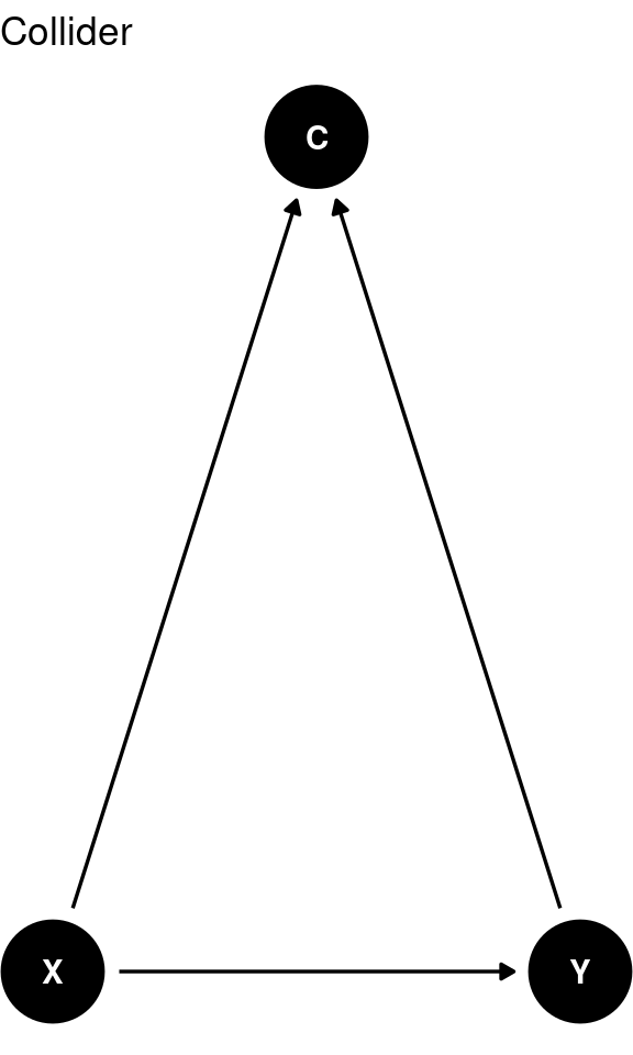
A collider is a variable that is influenced by both \(X\) and \(Y\). Conditioning on a collider can create a spurious association.
Avoid including colliders in the regression analysis. Including a collider can introduce bias and create a misleading relationship between \(X\) and \(Y\).
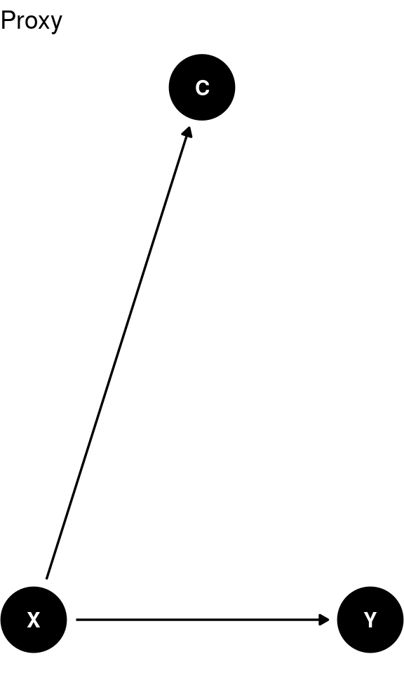
A proxy variable serves as a substitute for the variable of interest, often because the actual variable is difficult to measure.
Proxies can be included in the regression analysis as long as they are empirically valid representations of the variable they are intended to substitute and as long as measurement errors don’t exist. However, there is no need to include it as \(C\) does not have and impact on \(Y\) and if there is a measurement errors it can worsen your estimates.
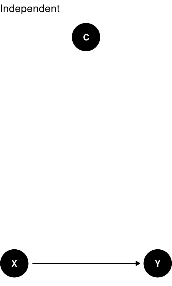
An independent is a variable that has no causal relation to either the outcome or predictor. Controlling for such a variable will have no systematic impact on the causal estimate.
8.4.3 Omitted variable bias (OVB) and ceteris paribus
From the Gauss-Markov theorem we know that if the OLS assumptions are fulfilled, the OLS estimator is (in the sense of smallest variance) the best linear conditionally unbiased estimator (BLUE). However, OLS estimates can suffer from omitted variable bias when any regressor, X, is correlated with any omitted variable that mat (OVB) ters for variable Y.
For omitted variable bias to occur, two conditions must be fulfilled:
- X is correlated with the omitted variable.
- The omitted variable is a determinant of the dependent variable Y.
In regression analysis, “ceteris paribus” is a Latin phrase that translates to “all other things being equal” or “holding everything else constant.” It is a concept used to examine the relationship between two variables while assuming that all other factors or variables remain unchanged.
When we say ceteris paribus in the context of regression analysis, we are isolating the effect of a specific independent variable on the dependent variable while assuming that the values of the other independent variables remain constant. By holding other variables constant, we can focus on understanding the direct relationship between the variables of interest.
For example, consider a regression analysis that examines the relationship between income (dependent variable) and education level (independent variable) while controlling for age, gender, and work experience. By stating ceteris paribus, we are assuming that age, gender, and work experience remain constant, and we are solely interested in understanding the impact of education level on income.
Exercise 8.2 Look at the Output
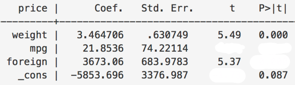
In Figure 8.5 you see an excerpt of a regression output taken from a statistical program named Stata. Some t-values and p-values are missing.
- Calculate the t-value of the coefficient
mpg. Is the coefficient at a level of \(\alpha=0.05\) statistically significant?
- Is the coefficient foreign at a level of \(\alpha=0.05\) statistically significant?
- Is the constant at a level of \(\alpha=0.05\) statistically significant?
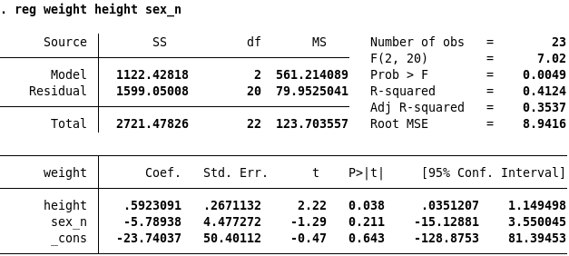
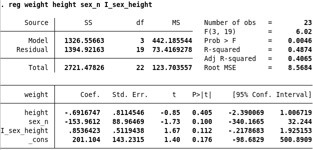
Exercise 8.3 Look at Stata Output
In Figure 8.6 you find two regression outputs from Stata. Try to interpret the p-values and the confidence intervals. How are the t-values calculated. Can you use the magic number 1.96 to say if a corresponding estimated coefficient is statistically significant, or not? Which estimated model is better?
Exercise 8.4 Explain the weight (Solutions online)
In the following exercise you need to use the programming language R.
- Write down your name, your matriculation number, and the date.
- Set your working directory.
- Clear your global environment.
- Load the following package:
tidyverse
library("tidyverse")The following table stems from a survey carried out at the Campus of the German Sport University of Cologne at Opening Day (first day of the new semester) between 8:00am and 8:20am. The survey consists of 6 individuals with the following information:
| id | sex | age | weight | calories | sport |
|---|---|---|---|---|---|
| 1 | f | 21 | 48 | 1700 | 60 |
| 2 | f | 19 | 55 | 1800 | 120 |
| 3 | f | 23 | 50 | 2300 | 180 |
| 4 | m | 18 | 71 | 2000 | 60 |
| 5 | m | 20 | 77 | 2800 | 240 |
| 6 | m | 61 | 85 | 2500 | 30 |
Data Description:
- id: Variable with an anonymized identifier for each participant.
- sex: Gender, i.e., the participants replied to be either male (m) or female (f).
- age: The age in years of the participants at the time of the survey.
- weight: Number of kg the participants pretended to weight.
- calories: Estimate of the participants on their average daily consumption of calories.
- sport: Estimate of the participants on their average daily time that they spend on doing sports (measured in minutes).
Which type of data do we have here? (Panel data, repeated cross-sectional data, cross-sectional data, time Series data)
Store each of the five variables in a vector and put all five variables into a dataframe with the title df. If you fail here, read in the data using this line of code:
df <- read_csv("https://raw.githubusercontent.com/hubchev/courses/main/dta/df-calories.csv")Show for all numerical variables the summary statistics including the mean, median, minimum, and the maximum.
Show for all numerical variables the summary statistics including the mean and the standard deviation, separated by male and female. Use therefore the pipe operator.
Suppose you want to analyze the general impact of average calories consumption per day on the weight. Discuss if the sample design is appropriate to draw conclusions on the population. What may cause some bias in the data? Discuss possibilities to improve the sampling and the survey, respectively.
The following plot visualizes the two variables weight and calories. Discuss what can be improved in the graphical visualization.
Create a scatterplot matrix to visualize relationships between all numerical variables in the dataset.
Calculate the Pearson Correlation Coefficient for the following pairs of variables:
caloriesandsportweightandcalories
This will help in understanding the strength and direction of the linear relationship between these variables.
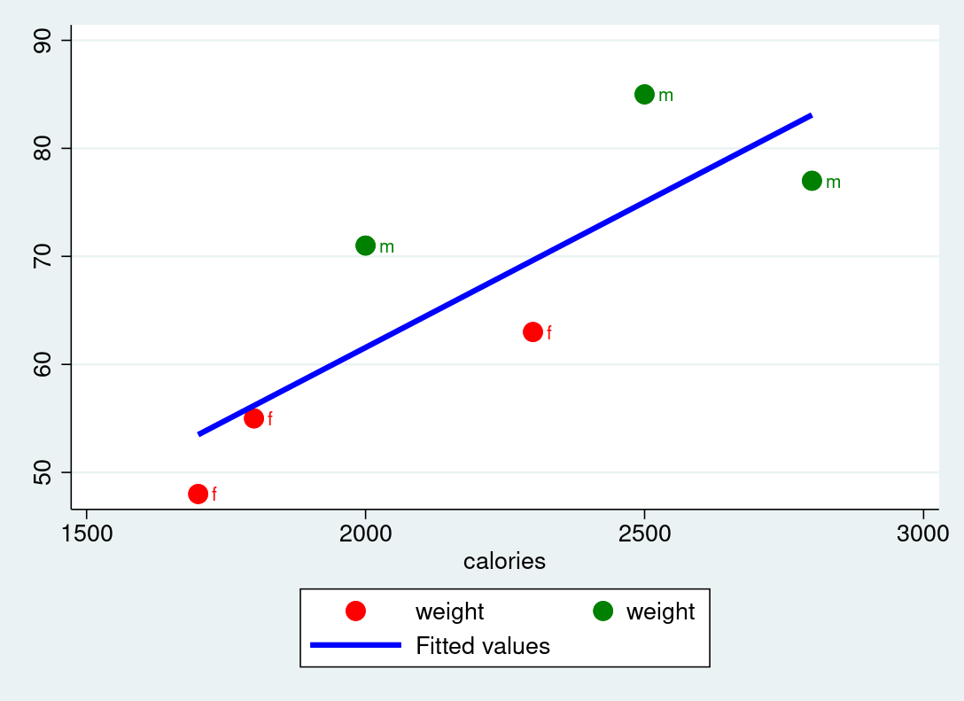
Generate a scatterplot with
weighton the y-axis andcalorieson the x-axis. Include a linear fit to the data and label the points with thesexvariable. This visualization can provide insights into the relationship between calorie consumption and weight, differentiated by gender.Estimate the following regression specification using the Ordinary Least Squares (OLS) method:
\[ weight_i=\beta_0+\beta_1 calories_i+ \epsilon_i \]
# OLS Regression
reg_base <- lm(weight ~ calories, data = df)
summary(reg_base)
Interpret the results. In particular, interpret how many kg the estimated weight increases—on average and ceteris paribus—if calories increase by 100 calories. Additionally, discuss the statistical properties of the estimated coefficient \(\hat{\beta_1}\) and the meaning of the Adjusted R-squared.
OLS estimates can suffer from omitted variable bias. State the two conditions that need to be fulfilled for omitted bias to occur.
Discuss potential confounding variables that may cause omitted variable bias. Given the dataset above how can some of the confounding variables be controlled for?
Warning: `install_github()` was deprecated in devtools 2.5.0.
ℹ Please use pak::pak("user/repo") instead.
Huber, S. (2025). How to use R for data science: Lecture notes. https://hubchev.github.io/ds/
Huntington-Klein, N. (2023). The effect: An introduction to research design and causality. CRC Press. https://theeffectbook.net