Appendix A — Solutions to exercises

Solution A.1. Exchange currencies (Exercise 1.2)

The equivalent amount in Euros for exchanging 500 US Dollars at the initial exchange rate of (1.20 , ) is given by: \[ \text{Equivalent Euros} = \frac{500 \, \text{USD}}{1.20 \, \text{USD/EUR}} \]
If the exchange rate changes to (1.15 , ), the new equivalent amount in Euros is: \[ \text{New Equivalent Euros} = \frac{500 \, \text{USD}}{1.15 \, \text{USD/EUR}} \]
The equivalent amount in US Dollars for spending 1,000 Euros at the initial exchange rate is: \[ \text{Equivalent USD} = 1,000 \, \text{EUR} \times 1.20 \, \text{USD/EUR} \]
If the European tourist exchanges their money at the changed rate of (1.15 , ), the new equivalent amount in US Dollars is:

\[ \text{New Equivalent USD} = 1,000 \, \text{EUR} \times 1.15 \, \text{USD/EUR} \]

Solution A.2. Big Mac Index (Exercise 1.8)

Please take part in the discussion in class.
Please take part in the discussion in class.
The exchange rate of Euros to Swiss Francs in direct quotation is: \[E^{\frac{\text{ EUR}}{\text{ CHF}}}=\frac{4.56 \text{ EUR}}{4.75 \text{ USD}} \cdot \frac{6.57 \text{ USD}}{6.50 \text{ CHF}} = \frac{29.9592 \text{ EUR}}{30.875 \text{ CHF}} \approx 0.9703 \frac{\text{ EUR}}{\text{ CHF}}\] and in indirect quotation: \[E^{\frac{\text{ CHF}}{\text{ EUR}}} \approx 1.0305 \frac{\text{ CHF}}{\text{ EUR}}.\] That means, we have to pay about 0.97 Euro for one Swiss Franc or one Euro costs about 1.03 Swiss Franc.
To exchange 100 Euro to Swiss Francs, we need to calculate \[100 \text{ EUR} \cdot 1.0305 \frac{\text{ CHF}}{\text{ EUR}} \approx 108.1428 \text{ CHF}\]
Here are the answers:
1. is false: The price of a Big Mac in $ is different across countries.
2. is correct.
3. is false: 1 Ruble costs 0.0160 Dollar: \[ \frac{2.09\text{ USD}}{130 \text{ RUB}} = 0.016\frac{\text{ USD}}{\text{RUB}}.\]
4. is incorrect: \[ \underbrace{\frac{6.65 \text{ CAD}}{5.08 \text{ USD}}}_{\approx 1.309}\cdot \underbrace{\frac{4.75 \text{ USD}}{4.56 \text{ EUR}}}_{\approx 1.0416} \approx 1.36\frac{\text{ CAD}}{\text{EUR}}. \]
5. is incorrect: \[ \frac{6.05 \text{ CAD}}{5.08 \text{ USD}} \approx 0.76 \frac{\text{ CAD}}{\text{ USD}}. \] Thus, with one Canadian Dollar you can buy 0.76 U.S. Dollar.

Solution A.3. Big Mac Index (Exercise 1.4)

International arbitrage strategy
- Strategy: Buy 50 units of good 08/15 in Germany for $2 each with your $100. Then, sell these units in Switzerland or the USA for $6 each, making a total of $300. This is a classic arbitrage strategy.
- Impact on Prices: Consider that you repeat that winning strategy to buy in Germany and sell in some other country, prices will change: The increased demand in Germany will cause the price there to rise, while the increased supply in Switzerland and the USA will cause the price to drop. Eventually, the price differences will equalize, eliminating the arbitrage opportunity.
Calculating exchange rates
- USD to EUR: $\frac{4 USD}{2 EUR} = 2\frac{USD}{EUR}$
- EUR to USD: $0.5 \frac{EUR}{USD}$
- USD to CHF: $\frac{2}{3} \frac{USD}{CHF}$
- CHF to USD: $1.5 \frac{CHF}{USD}$
- CHF to EUR: $\frac{4}{3} \frac{CHF}{USD}$
- EUR to CHF: $0.75 \frac{EUR}{USD}$

Solution A.4. Exchange rates and where to invest (Exercise 1.6)

Rate of return in the EU is 1 percent and hence you will have 10,100 in 2023. Rate of return in the US is about 0.62 percent: \[ 10000\text{€} \cdot \frac{1 \$}{0.93 \text{€}}\cdot 1.02 \cdot \frac{1 \text{€}}{1.09 \$}= 10062.1485 \text{€} \] Thus, it is better to invest in Europe.
In 2022 you have to pay 93 Cent for a dollar and in 2023 you expect to pay about 91 Cent for a dollar. Thus, you expect the Euro to appreciate.

Solution A.5. Turkey vs. Germany (Exercise 1.7)

When focusing solely on the interest rate, investing in Turkey appears more advantageous. However, if we consider only the development of the exchange rate, investing in Germany becomes more appealing due to the Euro appreciating relative to the Lira from period $t-1$ to $t$. Therefore, it’s essential to calculate the return on investment to determine which of the two effects predominates. This can be done in three different ways:
(Exact) calculation method in four steps:
```
 1. exchange € to ₺ in t-1:
```
\[ 100\text{€}\cdot E^{\text{₺}/\text{€}}_{t-1}= 100\text{€} \cdot 7\frac{\text{₺}}{\text{€}}=700\text{₺} \] 2. invest in either Germany or Turkey: \[GER \rightarrow 100\text{€}\cdot (1+0.01)=101\text{€}\] \[TUR\rightarrow 700\text{₺}\cdot(1+0.1)=770\text{₺}\] 3. re-exchange to : \[770\text{₺}\cdot E^{\text{€}/\text{₺}}_{t}= 770\text{₺}\cdot\frac{1 \text{€}}{7\frac{1}{10}\text{₺}}=\frac{7700}{71}\approx 108.4507\] 4. calculate the return on investment, $r$: \[\begin{align*} r_{GER}=&0.01\\ r_{TUR}=&\frac{108.4507-100}{100}=0.084507 \end{align*}\] Answer: The return on investment is lower in Germany. Thus, it is superior to invest the 100€ in Turkey.

(Exact) Calculation method in one step: \[\begin{align*} \overbrace{r}^{\text{rate of return}}=& \frac{I^{\text{€}}_t-I_{t-1}^{\text{€}}}{I_{t-1}^{\text{€}}} \end{align*}\] with $I^{\text{€}}_{t}=\overbrace{I^{\text{€}}_{t-1}}^{\text{investment in t-1}}\cdot \overbrace{E^{\text{₺}/\text{€}}_{t-1}}^{\text{exchange rate in t-1}}\cdot \overbrace{(1+i)}^{1+ \text{interest rate}}\cdot \overbrace{E^{\text{€}/\text{₺}}_{t}}^{\text{exchange rate in t}}$ \[\begin{align*} TUR\rightarrow I_{t}^{\text{€}}=&100\text{€}\cdot 7\frac{\text{₺}}{\text{€}}\cdot (1+0.1)\cdot\frac{1\text{€}}{7.1\text{₺}}=108.4507 \rightarrow r_{TUR}=0.084507\\ GER\rightarrow I_{t}^{\text{€}}=& 100\text{€} \cdot 1 \cdot (1+0.01)\cdot 1 = 101\text{€}\rightarrow r_{GER}=0.01 \end{align*}\]
(Approximative) calculation method: Steps a) to c) can be summarized as two rates of changes: \[\begin{align*} \underbrace{r'}_{\text{approximative rate of return}}=&\underbrace{i}_{\text{interest rate}}+\underbrace{w}_{\text{rate of depreciation}}\\ \text{with}\quad w=&\frac{E^{\text{€}/\text{₺}}_{t}}{E^{\text{€}/\text{₺}}_{t-1}}-1 \end{align*}\] \[\begin{align*} r'_{GER}=&0.01\\ r'_{TUR}=&0.1+\frac{\frac{10}{71}}{\frac{10}{70}}-1=0.1+\frac{700}{710}-1=0.1-\frac{10}{710}=\frac{61}{710}\approx 0.08591 \end{align*}\]

Both investments are equal profitable if \[r_{GER}=r_{TUR}.\] Given the information in period $t-1$, the exact exchange rate in period $t$ that makes investments are equal profitable, $E^{\text{€}/\text{₺}*}_{t}$, is calculated as follows: \[\begin{align*} I^{\text{€}}_{t}&=I^{\text{€}}_{t-1} E^{\text{₺}/\text{€}}_{t-1} (1+i) E^{\text{€}/\text{₺} *}_{t}\\ \Leftrightarrow E^{\text{€}/\text{₺}*}_{t}&= \frac{I^{\text{€}}_{t}}{(I^{\text{€}}_{t-1} E^{\text{₺}/\text{€}}_{t-1} (1+i))}=\frac{101}{(100\cdot 7 \cdot 1.1)}=\frac{101}{770}\approx 0.1311 \end{align*}\]

The approximate exchange rate in period $t$ that makes investments are equal profitable, $E^{\text{€}/\text{₺}*'}_{t}$, is calculated as follows: \[\begin{align*} r_{GER}=&i_{TUR}+\frac{E^{\text{€}/\text{₺}*'}_{t}}{E^{\text{€}/\text{₺}}_{t-1}}-1\\ \Leftrightarrow r_{GER}-i_{TUR}+1=&\frac{E^{\text{€}/\text{₺}*'}_{t}}{E^{\text{€}/\text{₺}}_{t-1}}\\ \Leftrightarrow E^{\text{€}/\text{₺}*'}_{t}=& (r_{GER}-i_{TUR}+1)\cdot E^{\text{€}/\text{₺}}_{t-1}\\ \Leftrightarrow E^{\text{€}/\text{₺}*'}_{t}=& (0.01-0.1+1)\cdot \frac{1}{7}=\frac{91}{100}\cdot \frac{1}{7}=\frac{91}{700}=0.13 \end{align*}\] Let us proof our results by re-calculating the rate of return for an investment in Turkey with $E^{\text{€}/\text{₺}*}_{t}$ and $E^{\text{€}/\text{₺}*'}_{t}$: \[\begin{align*} r'_{TUR}=&0.1+\frac{\frac{91}{700}}{\frac{1}{7}}-1=\frac{637}{700}-0.9=0.01\\ I_{t}^{\text{€}*}=&100\text{€}\cdot 7\frac{\text{₺}}{\text{€}}\cdot (1+0.1)\cdot \frac{91}{700}\frac{\text{€}}{\text{₺}}= \frac{70070}{700}=100.1\\ \rightarrow r_{TUR}^*=&0.01 \end{align*}\]

The ₺ must appreciate in t-1 since it is more profitable to exchange € to store the asset value in Turkey. That means the demand curve in the FOREX shifts upwards till the exchange rate equals the exchange rate that makes both investments equal profitable and hence nobody has an incentive to demand more ₺ for the given exchange rate $E^{\text{€}/\text{₺}*}_{t}$ as calculated above.

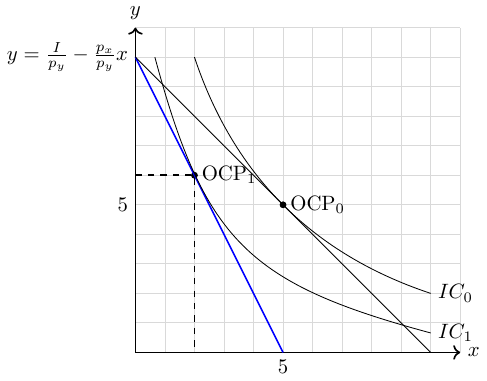
Solution A.6. Terms of trade (Exercise 2.2)

The new point of optimal consumption $OCP_1$ at $(x=2,y=6)$ illustrates that an increase in the price of good $x$ leads consumers to substitute good $x$ and consume more of good $y$ but less of good $x$.

The terms of trade are now $\frac{p_x}{p_y}=2$. That is, consumers are willing to give up 1 unit of good $x$ to receive 2 units of good $y$. The budget line is drawn in blue.

Figure A.1: Optimal consumption point after price increase

Solution A.7. Gains of small economies (Exercise 2.4)

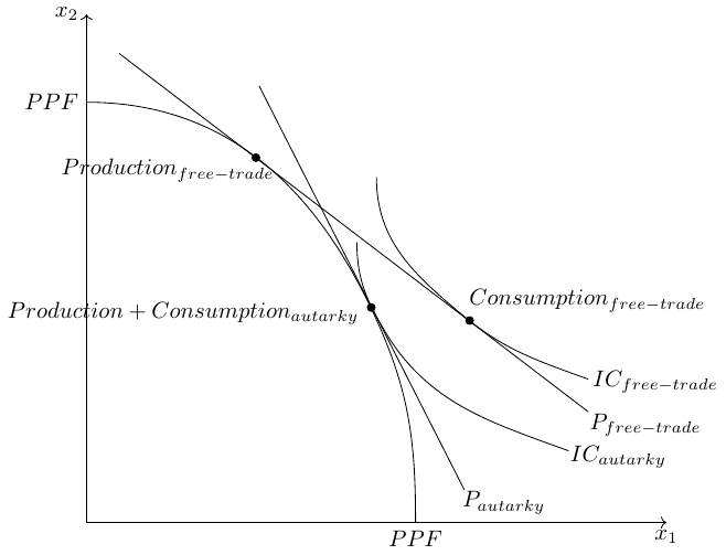
As visualized in Figure A.2, the indifference curve under free trade lies above the IC under autarky. This reflects the higher utility level under free trade.

Solution A.8. Comparative advantage and opportunity costs (Exercise 2.6)

Country A has an absolute advantage in producing both goods as \[ a_y^A=1<3=a_y^B \] and \[ a_x^A=2<4=a_x^B \]
Solution is shown in the lecture.
Opportunity cost is the value of what you lose when choosing between two or more options. Alternative definition: Opportunity cost is the loss you take to make a gain, or the loss of one gain for another gain.
If A wants top produce one unit more of good $y$ it has to give up $\frac{1}{2}$ units of good $x$.
If A wants top produce one unit more of good $x$ it has to give up $2$ units of good $y$.
If B wants top produce one unit more of good $y$ it has to give up $\frac{3}{4}$ units of good $x$.
If A wants top produce one unit more of good $x$ it has to give up $\frac{4}{3}$ units of good $y$.

opportunity costs of producing …	A	B
…1 unit of good $y$	$\frac{a_y^A}{a_x^A}=\frac{1}{2}=0.5$ (good x)	$\frac{a_y^B}{a_x^B}=\frac{3}{4}$ (good x)
…1 unit of good $x$	$\frac{a_x^A}{a_y^A}=\frac{2}{1}=2$ (good y)	$\frac{a_x^B}{a_y^B}=\frac{4}{3}=$ (good y)

Country A has a comparative advantage in producing good $y$.
Country B has a comparative advantage in producing good $x$.

Solution A.9. The best industry is not competitive (Exercise 2.7)

opportunity costs of producing…	Person A	Person B
…1 unit of good y:	a_y^A/a_xA = 1/2 = 0.5 (good x)	a_y^B/a_xB = 0.4/0.4 = 1 (good x)
…1 unit of good x:	a_x^A/a_yA = 2/1 = 2 (good y)	a_x^B/a_yB = 0.4/0.4 = 1 (good y)

Thus, A has a comparative advantage in producing good $y$ and B has a comparative advantage in producing good $x$. This seems to be counterintuitive as B can produce faster anything and everybody else.

When looking on input coefficients, we get \[ \frac{a^A_y}{a^A_x}=\frac{10}{12} < \frac{9}{10}=\frac{a^B_y}{a^B_x} \] which gives us the same comparative advantages as described above.

To become an exporter of $y$, B needs to have lower opportunity costs in the production of $y$ than A. This can happen by becoming more productive in producing $y$ **and/or} by becoming ‘slower’ in producing good $x$ so that $\frac{a_y^B}{a_x^B}<\frac{10}{12}$

Solution A.10. Comparative advantage and input coefficients (Exercise 2.8)

Country B has an absolute advantage in producing both goods.
Country A has a comparative advantage in producing good $y$.
Country B has a comparative advantage in producing good $x$.

Solution A.11. Comparative advantage: Germany and Bangladesh (Exercise 2.9)

Germany has an absolute advantage in the production of the three goods because it labor input coefficients are smaller in all three goods.
Since $p^{m/s}_B=\frac{100}{10000}<p^{m/s}_G=\frac{5}{50}$ Bangladesh has a comparative advantage in producing machines and Germany has a comparative advantage in producing ships.
Since $p^{m/c}_B=\frac{100}{50}>p^{m/c}_G=\frac{5}{3}$ Bangladesh has a comparative advantage in producing clothes and Germany has a comparative advantage in producing machines.
Since $p^{s/c}_B=\frac{10000}{50}>p^{s/c}_G=\frac{50}{3}$ Bangladesh has a comparative advantage in producing clothes and Germany has a comparative advantage in producing ships.
Germany has a clear comparative advantage in producing ships and hence will export ships. Moreover, Germany has a clear comparative disadvantage in producing cloth and will definitely import clothes.

Solution A.12. Multiple choice: Ricardian model (Exercise 2.10)

Choices b) and c) are correct.

Solution A.13. Ricardian Model again (Exercise 2.11)

and d) are true.

Solution A.14. Bikes and bike tires (Exercise 2.12)

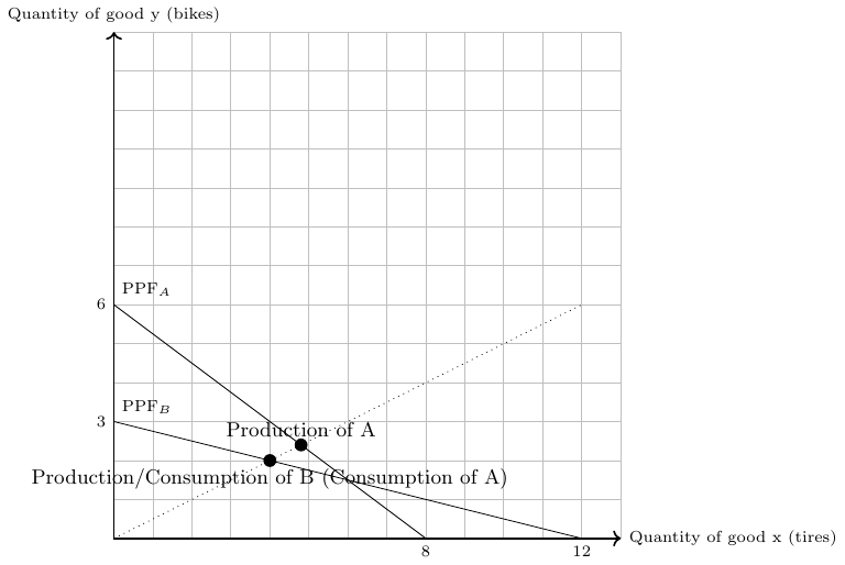
Both countries can consume 2 complete bikes, see Figure A.3.

Figure A.3: Production and consumption in A and B

	Country A	Country B
Good $y$ (bikes)	24:6=4	24:3=8
Good $x$ (bike tires)	24:8=3	24:12=2

If we assume that both countries specialize completely in the production of the good at which they have a comparative advantage and trade is allowed and free of costs, then

country A produces 6 units of bikes and 0 units of tires and
country B produces 0 units of bikes and 12 units of tires.

Moreover, since both countries aim to consume complete bikes, i.e., one bike with two tires,

country A exports 3 units of bikes and imports 6 units of tires and
country B exports 6 units of tires and imports 3 units of bikes.

Under free trade

country A can consume 3 complete bikes and
country B can consume 3 complete bikes.

Solution A.15. Ricardian model MC (Exercise 2.13)

a), b), and e) are correct statements.

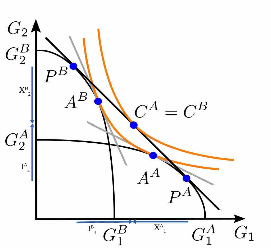
Solution A.16. HO-Model in one figure (Exercise 2.15)

Two identical countries (A and B) have different initial factor endowments. I assume that country A is abundantly endowed with the production factor that is intensively used in the production of good 1, the reverse holds for country B. Thus, the two solid black lines in Figure A.4 represents the respective production possibility frontier curves. The orange lines represents the respective indifference curves. Autarky equilibria are marked with $A^{A}$ and $A^{B}$, respectively. The production points in trade equilibrium are marked with $P^A$ and $P^B$, the consumption point of both countries is in $C^A=C^B$. Thus, production and consumption points are divergent. The indifference curve under free trade is clearly above the other indifference curve in autarky. The solid black line that is tangient to the consumption point under free trade represents the utility maximizing world market price under free trade. The exports, $X$, and imports; $I$, are denotes correspondingly to the goods and country names.

Solution A.17. Multiple choice: HO-Model (Exercise 2.16)

Answer a) is correct.

opportunity costs of producing …	A	B
…1 unit of good \(y\)	\(\frac{a_y^A}{a_x^A}=\frac{1}{2}=0.5\) (good x)	\(\frac{a_y^B}{a_x^B}=\frac{3}{4}\) (good x)
…1 unit of good \(x\)	\(\frac{a_x^A}{a_y^A}=\frac{2}{1}=2\) (good y)	\(\frac{a_x^B}{a_y^B}=\frac{4}{3}=\) (good y)