5 What can go wrong?
In empirical research, identification refers to the process of establishing a clear and logical relationship between a cause and an effect. This involves demonstrating that the cause is responsible for the observed effect, and that there are no other factors that could potentially explain the effect. The goal of identification is to provide strong evidence that a particular factor is indeed the cause of a particular outcome, rather than simply coincidentally happen. In order to identify a cause-and-effect relationship, researchers can use experimental or non-experimental, that is, observational data, or both. Section 5.1 to Section 5.3 will explain some difficulties researchers must face when they aim to find empirical evidence on causal effects.
5.1 Pitfalls
This section highlights some common pitfalls when dealing with data. Being aware of these pitfalls helps build best practices to maintain the integrity of analyses and visualizations. More pitfalls and explanations can be found in the excellent book by Jones (2020). I recommend reading this book.
Epistemic errors occur when there are mistakes in our understanding and conceptualization of data. These errors arise from cognitive biases, misunderstandings, and incorrect assumptions about the nature of data and the reality it represents. Recognizing and addressing these errors is crucial for accurate data analysis and effective decision-making.
One significant type of epistemic error is the data-reality gap, which refers to the difference between the data we collect and the reality it is supposed to represent. For example, a survey on customer satisfaction that only includes responses from a self-selected group of highly engaged customers may not accurately reflect the overall customer base. To avoid this specific pitfall, it is essential to ensure that your data collection methods are representative and unbiased, and to validate your data against external benchmarks or additional data sources.
To avoid epistemic errors, critically assess your assumptions, methodologies, and interpretations. Engage in critical thinking by regularly questioning your assumptions and seeking alternative explanations for your findings. Employ methodological rigor by using standardized and validated methods for data collection and analysis. Engage with peers to review and critique your work, providing a fresh perspective and identifying potential biases. Finally, stay updated with the latest research and best practices in your field to avoid outdated or incorrect methodologies.
Another common epistemic error involves the influence of human biases during data collection and interpretation. Known as the all too human data error, this occurs when personal biases or inaccuracies affect the data. An example would be a researcher’s personal bias influencing the design of a study or the interpretation of its results. To mitigate this, implement rigorous protocols for data collection and analysis, and consider using double-blind studies and peer reviews to minimize bias.
Inconsistent ratings can also lead to epistemic errors. This happens when there is variability in data collection methods, resulting in inconsistent or unreliable data. For example, different evaluators might rate the same product using different criteria or standards. To avoid this issue, standardize data collection processes and provide training for all individuals involved in data collection to ensure consistency.
Understanding and addressing epistemic errors can significantly improve the reliability and accuracy of your data analyses, leading to better decision-making and more trustworthy insights.
5.2 Correlation does not imply causation
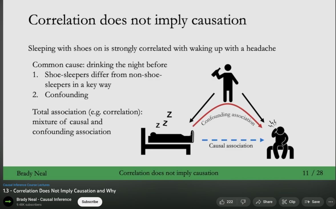
Correlation refers to a statistical relationship between two variables, where one variable tends to increase or decrease as the other variable also increases or decreases. However, just because two variables are correlated does not necessarily mean that one variable causes the other. This is known as the correlation does not imply causation principle.
For example, across many areas the number of storks is correlated with the birth rate of babies (see Matthews, 2000). However, this does not mean that the presence of storks causes an increase in the birth rate. It is possible that both the number of storks and the number of babies born are influenced by other factors, such as the overall population density or economic conditions in the area.
Therefore, it is important to carefully consider all possible explanations (confounders) for a correlation and to use data to disentangle the true cause-and-effect relationship between variables.
1 Source: https://youtu.be/DFPm_a-_uJM
Watch the video of Brady Neal’s lecture Correlation Does Not Imply Causation and Why. Alternatively, you can read chapter 1.3 of his lecture notes (Neal, 2020) which you find here.
5.3 Simpsons Paradox
5.3.1 A simple representation
Suppose you receive the following data from two hospitals, A and B, as shown in Table Table 5.1:
| Survived (A) | Treated (A) | Survival Rate (A) | Survived (B) | Treated (B) | Survival Rate (B) |
|---|---|---|---|---|---|
| 68 | 100 | 0.68 | 83 | 100 | 0.83 |
At first glance, hospital B appears to be more succesful, as its survival rate is higher than hospital A’s. You discover that the two hospitals use different treatment approaches: hospital A applies the most advanced methods, while hospital B relies on more traditional techniques. Does this mean traditional—and likely less expensive—methods are superior? Not necessarily.
For example, let’s assume the hospitals differ not only in their treatments but also in their patient demographics, as shown in Table Table 5.2: In hospital A, 80% of patients were aged 65 and older, whereas in hospital B, only 10% were in this age group. If you examine the survival rates within each age group separately, hospital A outperforms hospital B among older patients and is equally effective among younger patients. With this more detailed data, hospital A’s methods actually appear more successful.
This phenomenon, where conclusions from aggregated data contradict those from disaggregated data, is known as Simpson’s Paradox.
| Age group | Survived (A) | Treated (A) | Survival Rate (A) | Survived (B) | Treated (B) | Survival Rate (B) |
|---|---|---|---|---|---|---|
| younger than 65 years | 18 | 20 | 0.90 | 81 | 90 | 0.9 |
| 65 years and older | 50 | 80 | 0.625 | 2 | 10 | 0.10 |
| Overall | 68 | 100 | 0.68 | 83 | 100 | 0.83 |
5.3.2 A real case
2 Source: The photography is public domain and stems from the Library of Congress Prints and Photographs Division Washington, see: http://hdl.loc.gov/loc.pnp/pp.print.
Discrimination is bad. Whenever we see it, we should try to find ways to overcome it. De jure segregation mandated the separation of races by law is clearly discriminatory. Other forms of discrimination, however, are often more difficult to spot and as long we don’t have good evidence for discrimination, we should not judge prematurely. That means, we should be sure that we see an act of making unjustified distinctions between individuals based on some categories to which they belong or perceived to belong. For example, if men and women are treated differently without an acceptable reason, we consider it discriminative.
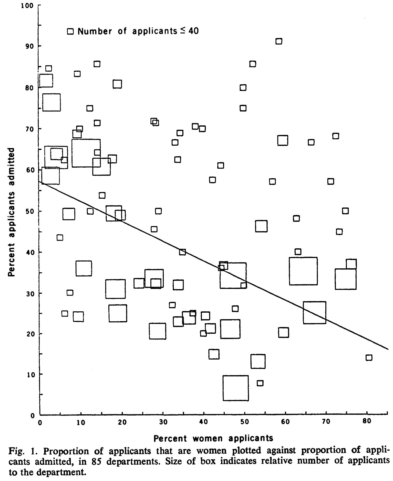
However, as the following example discussed in Bickel et al. (1975) will show, it is often challenging to identify discrimination. In 1973, UC Berkeley was accused of discrimination because it admitted only 35% of female applicants but 44% of male applicants overall. The difference was statistical significant and based on that many people protested claiming justice and equality. However, it turned out that the selection of students was not discriminative against women but against men. Accordingly to Bickel et al. (1975) the different overall admission rates can be largely explained by a “tendency of women to apply to graduate departments that are more difficult for applicants of either sex to enter” (Bickel et al., 1975, p. 403). Figure Figure 5.4 taken from Bickel et al. (1975, p. 403) visualizes this fact. Looking on the decisions within the departments seperately, there is even a “statistically significant bias in favor of women” (Bickel et al., 1975, p. 403).
3 Source: Bickel et al. (1975, p. 403)
Here is a summary of Bickel et al. (1975, p. 403):
“Examination of aggregate data on graduate admissions to the University of California, Berkeley, for fall 1973 shows a clear but misleading pattern of bias against female applicants. Examination of the disaggregated data reveals few decision-making units that show statistically significant departures from expected frequencies of female admissions, and about as many units appear to favor women as to favor men. If the data are properly pooled, taking into account the autonomy of departmental decision making, thus correcting for the tendency of women to apply to graduate departments that are more difficult for applicants of either sex to enter, there is a small but statistically significant bias in favor of women. The graduate departments that are easier to enter tend to be those that require more mathematics in the undergraduate preparatory curriculum. The bias in the aggregated data stems not from any pattern of discrimination on the part of admissions committees, which seem quite fair on the whole, but apparently from prior screening at earlier levels of the educational system. Women are shunted by their socialization and education toward fields of graduate study that are generally more crowded, less productive of completed degrees, and less well funded, and that frequently offer poorer professional employment prospects.”
The UC Berkley case is just one of many examples to illustrate that uniformity of group assignment of individuals is a necessary condition to ensure that pooling of data does not lead to misleading conclusions when using statistics. The phenomenon of obtaining different results depending on whether one considers the data pooled or unpooled is often referred to as the Simpson Paradox.
In Section 8.2.1, we will revisit this paradox, defining it as a situation where the association between two variables can be reversed in an regression analysis if a third variable is taken into account (controlled for).


