Appendix B — Exam(ple) questions
Exercise B.1 OLS method
In the course, we have discussed the OLS method.
- What does OLS stand for?
- Explain the OLS method for a simple linear regression using a two-dimensional plot.
OLS stands for Ordinary Least Squares.
In the OLS method, the goal is to find the best-fitting line through a set of data points. More generally, it aims to make the best prediction by minimizing the sum of the squared residuals which are the vertical distances between each data point (\(y_i\)) and the predicted value on the line (\(y_i^*\)). The so-called residual is the difference between the observed value (\(y_i\)) and the value predicted by the regression line (\(y_i^*\)). The corresponding sketch is shown in Figure 8.1.
Exercise B.2 Correlation
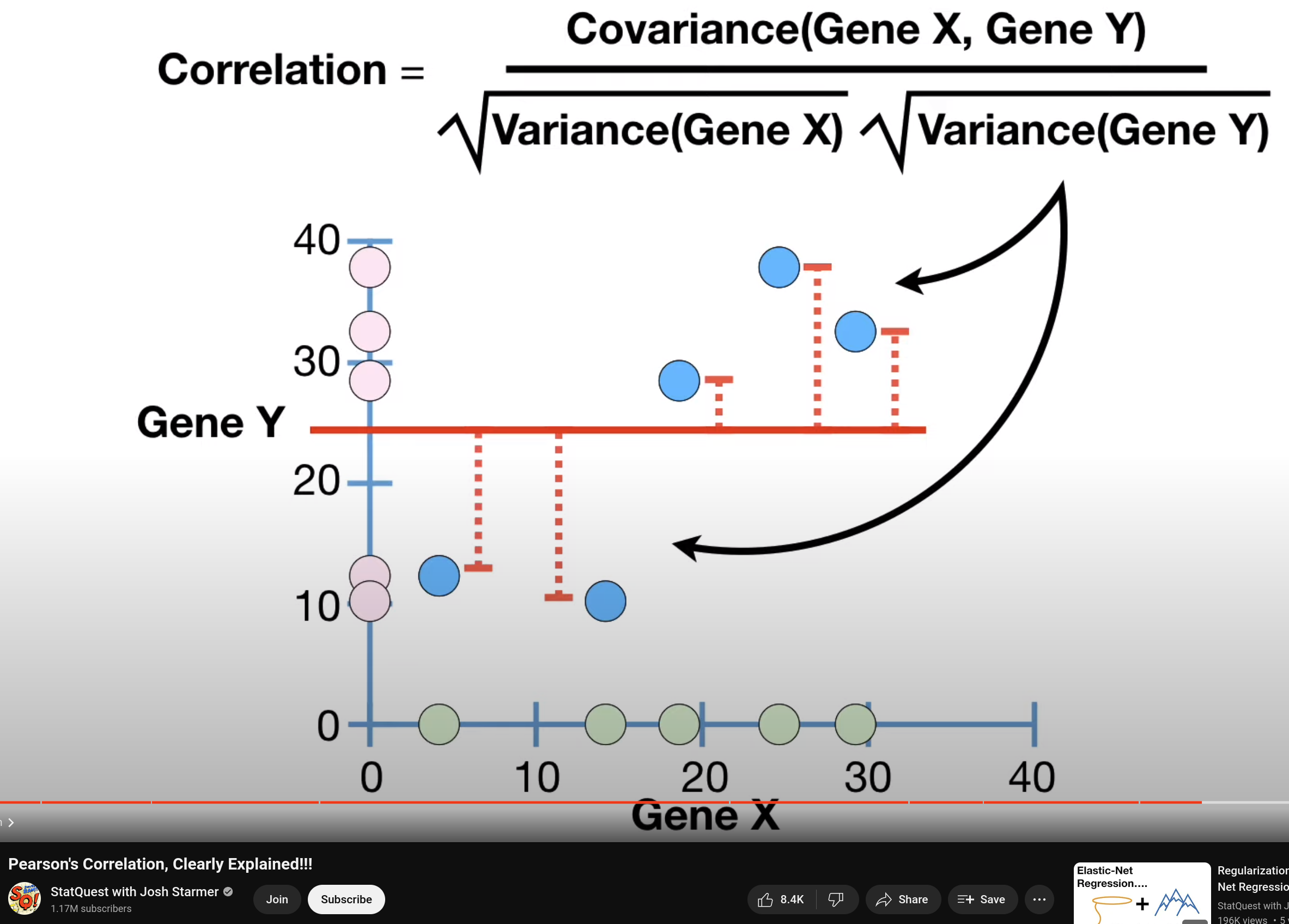
Figure B.1 shows a screenshot of Josh Starmer’s explanation of the correlation coefficient. The video was linked in the lecture notes and watched during the lecture.
Source: StatQuest with Josh Starmer
Explain in detail why the covariance is divided by the denominator shown in the figure.
Discuss the interpretation of positive and negative values of the correlation coefficient. What does a correlation coefficient of zero mean?
Comment the following statement:
“A correlation coefficient of zero is evdience that the the two variables are not associated.”
Explain the limitations of the correlation coefficient for empirical research in great detail.
The correlation coefficient measures the direction of the linear relationship between two variables. It is calculated using the covariance of the variables divided by the product of their standard deviations.
By dividing the covariance by the product of the standard deviations of the two variables, we standardize the measure. This ensures that the correlation coefficient is dimensionless and falls within a fixed range regardless of the units of the original variables.
In contrast to the covariance, the correlation coefficient allows for comparison of the linear relationships between different pairs of variables because the denominator normalizes the covariance (from -1 to 1). Without this normalization, the magnitude of the covariance is influenced by the scales of the variables. Normalization removes the dependency on the scales, providing a pure measure of the linear relationship.
In summary, the covariance is divided by the product of the standard deviations to standardize, normalize, and make the measure dimensionless, allowing for meaningful and comparable interpretation of the linear relationship between the two variables.
The correlation coefficient provides a clearer interpretation: a correlation coefficient of 1 (-1) implies a perfect positive (negative) linear relationship, and 0 implies no linear relationship, that is, there is no consistent tendency for one variable to increase or decrease as the other variable changes.
In other words, a positive (negative) correlation coefficient indicates that as one variable increases, the other variable also tends to increase (decreases).
It’s essential to note that a correlation coefficient of zero does not necessarily mean there’s no relationship at all between the variables; it just implies that there’s no linear relationship. There could still be a nonlinear relationship or other forms of association between the variables.
The correlation coefficient is a limited indicator in empirical research, especially when the reasearch is interested in causality. In the following, I elaborate on some points in greater detail:
Causation vs. Correlation: The correlation coefficient measures the strength and direction of a linear relationship between variables but does not imply causation. Just because two variables are correlated does not mean that one causes the other. It’s essential to conduct further research to establish causation.
Nonlinear Relationships: The correlation coefficient only measures linear relationships between variables. It may not capture more complex relationships. Therefore, it’s possible for variables to have a significant relationship that is not detected by the correlation coefficient.
Outliers in the data can significantly influence the correlation coefficient. A few extreme data points can inflate or deflate the correlation coefficient, leading to misleading conclusions about the relationship between variables.
Confounding Variables: Correlation does not account for the effects of confounding variables, which can influence the relationship between the variables of interest. Failing to control for confounders can lead to spurious correlations or misinterpretation of results.
Sample Size: The reliability of the correlation coefficient depends on the sample size. Small sample sizes may not provide enough statistical power to detect significant correlations accurately. Additionally, large sample sizes can sometimes yield statistically significant correlations that are not practically meaningful.
These limitations highlight the importance of interpreting correlation coefficients cautiously and considering additional factors when drawing conclusions in empirical research.
Exercise B.3 Regression
- In class, we discussed the phrase `garbage in garbage out’. Explain what is meant by this.
- Explain what is meant with omitted variable bias and confounding variables in the multiple regression model.
