4  Statistics

Learning objectives

In this chapter, we will explore several key concepts essential for conducting empirical analysis through statistical inference. Specifically, we will cover:

  • The defining characteristics of a sample suitable for empirical analysis and statistical inference.
  • The distinction between a sample and a population, and why understanding this difference is critical.
  • How to identify biased samples and understand the implications of bias in empirical research.
  • The differences between random sampling and random assignment, including their respective roles in research.
  • Why a simple random sample is considered the gold standard in sampling methods due to its advantageous properties.
  • Various methods for data collection and drawing samples, highlighting the strengths and weaknesses of each approach.

4.1 Sampling

4.1.1 The Hite Report

In 1976, when the The Hite Report (see Hite, 1976) was published it instantly became a best seller. Hite used an individualistic research method. Thousands of responses from anonymous questionnaires were used as a framework to develop a discourse on human responses to gender and sexuality. The following comic concludes the main results.

Figure 4.1: The Hite (1976) Report
Figure 4.2: Comic on the Hite Report1

1 Picture is taken from https://www.theparisreview.org/blog/2017/07/21/great-moments-literacy-hite-report.

The picture of womens’ sexuality in Hite (1976) was probably a bit biased as the sample can hardly be considered to be a random and unbiased one:

Hite, S. (1976). The hite report. A nationwide study of female sexuality. New York: Dell.
  • Less than 5% of all questionnaires which were sent out were filled out and returned (response bias).
  • The questions were only sent out to women’s organizations (an opportunity sample).

Thus, the results were based on a sample of women who were highly motivated to answer survey’s questions, for whatever reason.

4.1.2 Sample design

In statistics and quantitative research methodology, a sample is a group of individuals or objects that are collected or selected from a statistical population using a defined procedure. The elements of a sample are called sample points, sampling units, or observations.

Usually, the population is very large, and therefore, conducting a census or complete enumeration of all individuals in the population is either impractical or impossible. Therefore, a sample is taken to represent a manageable subset of the population. Data is collected from the sample, and statistics are calculated to make inferences or extrapolations from the sample to the population.

In statistics, we often rely on a sample, that is, a small subset of a larger set of data, to draw inferences about the larger set. The larger set is known as the population from which the sample is drawn.

Researchers adopt a variety of sampling strategies. The most straightforward is simple random sampling. Such sampling requires every member of the population to have an equal chance of being selected into the sample. In addition, the selection of one member must be independent of the selection of every other member. That is, picking one member from the population must not increase or decrease the probability of picking any other member (relative to the others). In this sense, we can say that simple random sampling chooses a sample by pure chance. To check your understanding of simple random sampling, consider the following example. What is the population? What is the sample? Was the sample picked by simple random sampling? Is it biased?

4.1.2.1 Random sampling

Random sampling is a sampling procedure by which each member of a population has an equal chance of being included in the sample. Random sampling ensures a representative sample. There are several types of random sampling. In simple random sampling, not only each item in the population but each sample has an equal probability of being picked. In systematic sampling, items are selected from the population at uniform intervals of time, order, or space (as in picking every one-hundredth name from a telephone directory). Systematic sampling can be biased easily, such as, for example, when the amount of household garbage is measured on Mondays (which includes the weekend garbage). In stratified and cluster sampling, the population is divided into strata (such as age groups) and clusters (such as blocks of a city) and then a proportionate number of elements is picked at random from each stratum and cluster. Stratified sampling is used when the variations within each stratum are small in relation to the variations between strata. Cluster sampling is used when the opposite is the case. In what follows, we assume simple random sampling. Sampling can be from a finite population (as in picking cards from a deck without replacement) or from an infinite population (as in picking parts produced by a continuous process or cards from a deck with replacement).

In statistics, a simple random sample is a subset of individuals (a sample) chosen from a larger set (a population). Each individual is chosen randomly and entirely by chance, such that each individual has the same probability of being chosen at any stage during the sampling process, and each subset of k individuals has the same probability of being chosen for the sample as any other subset of k individuals.

The simple random sample has two important properties:

  1. UNBIASED: Each unit has the same chance of being chosen.
  2. INDEPENDENCE: Selection of one unit has no influence on the selection of other units.

Exercise 4.1 Random sampling (Solution 4.1)

  • What is meant by random sampling (simple random sample)?
  • What is its importance?
  • Why is having a large sample always better than having a small(er) one?

4.1.2.2 Other sampling methods

Systematic sampling

Systematic sampling (a.k.a. interval sampling) relies on arranging the study population according to some ordering scheme and then selecting elements at regular intervals through that ordered list. Systematic sampling involves a random start and then proceeds with the selection of every k\(^{th}\) element from then onwards.

Accidental sampling / opportunity sampling / convenience sampling

These sampling methods describe a type of nonprobability sampling which involves the sample being drawn from that part of the population which is close to hand. That is, a population is selected because it is readily available and convenient.

Stratified sampling

Since simple random sampling often does not ensure a representative sample, a sampling method called stratified random sampling is sometimes used to make the sample more representative of the population. This method can be used if the population has a number of distinct groups. In stratified sampling, you first identify members of your sample who belong to each group. Then you randomly sample from each of those subgroups in such a way that the sizes of the subgroups in the sample are proportional to their sizes in the population. Let`s take an example: Suppose you were interested in views of capital punishment at an urban university. You have the time and resources to interview 200 students. The student body is diverse with respect to age; many older people work during the day and enroll in night courses (average age is 39), while younger students generally enroll in day classes (average age of 19). It is possible that night students have different views about capital punishment than day students. If 70% of the students were day students, it makes sense to ensure that 70% of the sample consisted of day students. Thus, your sample of 200 students would consist of 140 day students and 60 night students. The proportion of day students in the sample and in the population (the entire university) would be the same. Inferences to the entire population of students at the university would therefore be more secure.

Cluster sampling

Sometimes it is more cost-effective to select respondents in groups (clusters) of similar respondents. Sampling is often clustered by geography, or by time periods.

4.1.2.3 Random assignment

In experimental research, populations are often hypothetical. For example, in an experiment comparing the effectiveness of a new anti-depressant drug with a placebo, there is no actual population of individuals taking the drug. In this case, a specified population of people with some degree of depression is defined and a random sample is taken from this population. The sample is then randomly divided into two groups; one group is assigned to the treatment condition (drug) and the other group is assigned to the control condition (placebo). This random division of the sample into two groups is called random assignment. Random assignment is critical for the validity of an experiment. For example, consider the bias that could be introduced if the first 20 subjects to show up at the experiment were assigned to the experimental group and the second 20 subjects were assigned to the control group. It is possible that subjects who show up late tend to be more depressed than those who show up early, thus making the experimental group less depressed than the control group even before the treatment was administered. In experimental research of this kind, failure to assign subjects randomly to groups is generally more serious than having a non-random sample. Failure to randomize (the former error) invalidates the experimental findings. A non-random sample (the latter error) simply restricts the generalizability of the results.

4.1.3 Sample size

The sample size is an important feature of any empirical study in which the goal is to make inferences about a population from a sample. In practice, the sample size used in a study is usually determined based on the cost, time, or convenience of collecting the data, and the need for it to offer sufficient statistical power.

Recall that the definition of a random sample is a sample in which every member of the population has an equal chance of being selected. This means that the sampling procedure rather than the results of the procedure define what it means for a sample to be random. Random samples, especially if the sample size is small, are not necessarily representative of the entire population.

Larger sample sizes generally lead to increased precision when estimating unknown parameters. For example, if we wish to know the proportion of a certain species of fish that is infected with a pathogen, we would generally have a more precise estimate of this proportion if we sampled and examined 200 rather than 100 fish. Several fundamental facts of mathematical statistics describe this phenomenon, including the law of large numbers and the central limit theorem.

Tip 4.1

The quality of data matters

A helpful slogan to keep in mind while scrutinizing statistical results is garbage in, garbage out. Regardless of how scientifically sound and visually appealing a statistic may appear, the formula used to derive it is oblivious to the quality of the data that underpins it. It is your responsibility to conduct a thorough examination. For example, if the data on which the statistic is based emanates from a biased sample (one that favors certain individuals over others), a flawed design, unreliable data-collection protocols, or misleading questions, the margin of error becomes bad. If the bias is sufficiently severe, the outcomes become worthless.

4.1.4 Sample errors

Read the following examples2:

2 The examples are taken from Lane (2023) and can be accessed here.

Lane, D. M. (2023). Introduction to statistics: Online statistics education: A multimedia course of study. Accessed January 30, 2023; Online Statistics Education: A Multimedia Course of Study. http://onlinestatbook.com

Example 1: You have been hired by the National Election Commission to examine how the American people feel about the fairness of the voting procedures in the U.S. Who will you ask?

It is not practical to ask every single American how he or she feels about the fairness of the voting procedures. Instead, we query a relatively small number of Americans, and draw inferences about the entire country from their responses. The Americans actually queried constitute our sample of the larger population of all Americans. The mathematical procedures whereby we convert information about the sample into intelligent guesses about the population fall under the rubric of inferential statistics. A sample is typically a small subset of the population. In the case of voting attitudes, we would sample a few thousand Americans drawn from the hundreds of millions that make up the country. In choosing a sample, it is therefore crucial that it not over-represent one kind of citizen at the expense of others. For example, something would be wrong with our sample if it happened to be made up entirely of Florida residents. If the sample held only Floridians, it could not be used to infer the attitudes of other Americans. The same problem would arise if the sample were comprised only of Republicans. __Inferential statistics are based on the assumption that sampling is random}. We trust a random sample to represent different segments of society in close to the appropriate proportions (provided the sample is large enough; see below).

Example 2: We are interested in examining how many math classes have been taken on average by current graduating seniors at American colleges and universities during their four years in school. Whereas our population in the last example included all US citizens, now it involves just the graduating seniors throughout the country. This is still a large set since there are thousands of colleges and universities, each enrolling many students. It would be prohibitively costly to examine the transcript of every college senior. We therefore take a sample of college seniors and then make inferences to the ntire population based on what we find. To make the sample, we might first choose some public and private colleges and universities across the United States. Then we might sample 50 students from each of these institutions. Suppose that the average number of math classes taken by the people in our sample were 3.2. Then we might speculate that 3.2 approximates the number we would find if we had the resources to examine every senior in the entire population. But we must be careful about the possibility that our sample is non-representative of the population. Perhaps we chose an overabundance of math majors, or chose too many technical institutions that have heavy math requirements. Such bad sampling makes our sample unrepresentative of the population of all seniors. To solidify your understanding of sampling bias, consider the following example. Try to identify the population and the sample, and then reflect on whether the sample is likely to yield the information desired.

Example 3: A substitute teacher wants to know how students in the class did on their last test. The teacher asks the 10 students sitting in the front row to state their latest test score. He concludes from their report that the class did extremely well. What is the sample? What is the population? Can you identify any problems with choosing the sample in the way that the teacher did?

In Example 3, the population consists of all students in the class. The sample is made up of just the 10 students sitting in the front row. The sample is not likely to be representative of the population. Those who sit in the front row tend to be more interested in the class and tend to perform higher on tests. Hence, the sample may perform at a higher level than the population.

Example 4: A coach is interested in how many cartwheels the average college freshmen at his university can do. Eight volunteers from the freshman class step forward. After observing their performance, the coach concludes that college freshmen can do an average of 16 cartwheels in a row without stopping.

In Example 4, the population is the class of all freshmen at the coach’s university. The sample is composed of the 8 volunteers. The sample is poorly chosen because volunteers are more likely to be able to do cartwheels than the average freshman; people who can’t do cartwheels probably did not volunteer! In the example, we are also not told of the gender of the volunteers. Were they all women, for example? That might affect the outcome, contributing to the non-representative nature of the sample.

Example 5: Sometimes it is not feasible to build a sample using simple random sampling. To see the problem, consider the fact that both Dallas and Houston are competing to be hosts of the 2012 Olympics. Imagine that you are hired to assess whether most Texans prefer Houston to Dallas as the host, or the reverse. Given the impracticality of obtaining the opinion of every single Texan, you must construct a sample of the Texas population. But now notice how difficult it would be to proceed by simple random sampling. For example, how will you contact those individuals who don’t vote and don’t have a phone? Even among people you find in the telephone book, how can you identify those who have just relocated to California (and had no reason to inform you of their move)? What do you do about the fact that since the beginning of the study, an additional 4,212 people took up residence in the state of Texas? As you can see, it is sometimes very difficult to develop a truly random procedure.

4.2 Descriptive statistics

Learning objectives:

  • Calculate and interpret the arithmetic mean, median, mode, range, variance, and standard deviation of a dataset.
  • Understand the concepts of skewness and kurtosis to describe the shape of data distribution.
  • Distinguish between standard deviation and standard error, and compute the standard error of the mean.
  • Learn the calculation and application of the coefficient of variation as a relative measure of variability.
  • Grasp the fundamentals of covariance and the Pearson correlation coefficient to measure the relationship between two variables.
  • Explore the Spearman rank correlation coefficient for non-parametric data analysis.
  • Apply these statistical measures to real-world datasets through exercises and supplementary video materials.

4.2.1 Univariate data

4.2.1.1 Arithmetic mean

The arithmetic mean (\(\bar{x}\)) is calculated as the sum of all the values in a dataset divided by the total number of values:

\[\bar{x} = \frac{{\sum_{i=1}^{n} x_i}}{n}\]

where \(\bar{x}\) represents the arithmetic mean, \(x_i\) represents each individual value in the dataset, and \(n\) represents the total number of values in the dataset.

4.2.1.2 Median

The median is the middle value of a dataset when it is sorted in ascending or descending order. If the dataset has an odd number of values, the median is the middle value. If the dataset has an even number of values, the median is the average of the two middle values.

4.2.1.3 Mode

The mode is the value or values that appear most frequently in a dataset.

4.2.1.4 Range

The range is the difference between the maximum and minimum values in a dataset.

\[ \text{{Range}} = \max(x_i) - \min(x_i) \]

where \(\text{{Range}}\) represents the range value, and \(x_i\) represents each individual value in the dataset.

4.2.1.5 Variance

The variance represents the average of the squared deviations of a random variable from its mean. It quantifies the extent to which a set of numbers deviates from their average value. Variance is commonly denoted as \(Var(X)\), \(\sigma^2\), or \(s^2\). The calculation of variance is as follows: \[ \sigma^2={\frac{1}{n}}\sum _{i=1}^{n}(x_{i}-\mu )^{2} \] However, it is better to use \[ \sigma^2={\frac{1}{n-1}}\sum _{i=1}^{n}(x_{i}-\mu )^{2}. \]

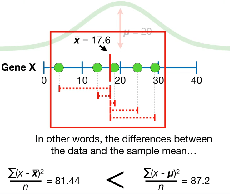
The use of \(n - 1\) instead of \(n\) in the formula for the sample variance is known as Bessel’s correction, which corrects the bias in the estimation of the population variance, and some, but not all of the bias in the estimation of the population standard deviation. Consequently this way to calculate the variance and hence the standard deviation is called the sample standard deviation or the unbiased estimation of standard deviation. In other words, when working with a sample instead of the full population the limited number of observations tend to be closer to the sample mean than to the population mean, see Figure 4.3. Bessels Correction takes that into account.

For a detailed explanation, you can watch the video by 
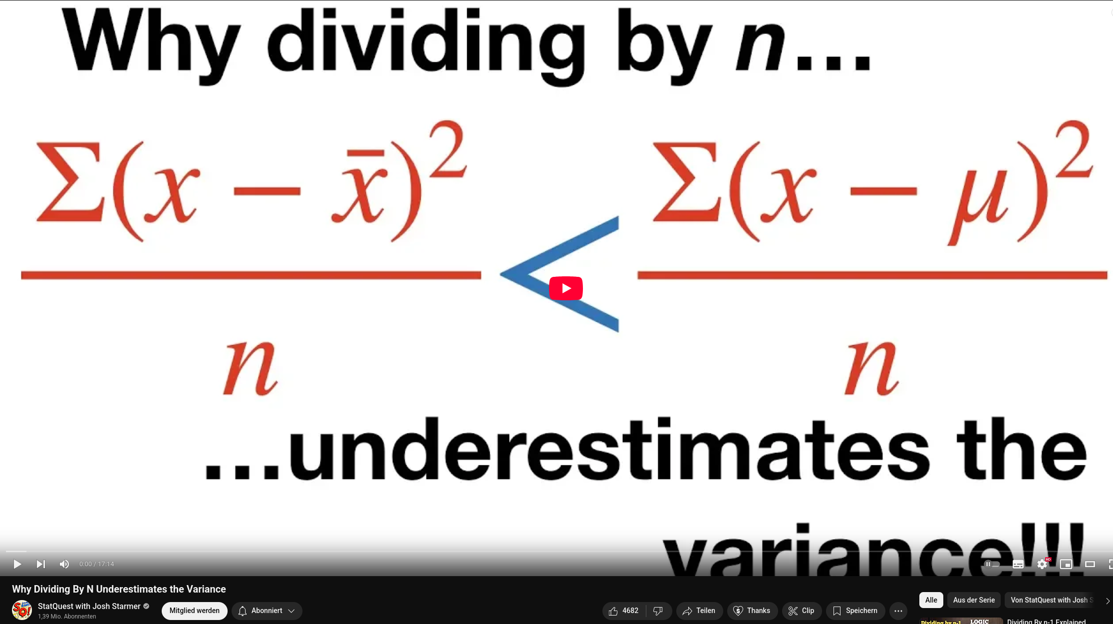
StatQuest with Josh Starmer: Why Dividing By N Underestimates the Variance

Figure 4.3: Bias when using the sample mean3

3 Picture is taken from the video https://youtu.be/sHRBg6BhKjI

4.2.1.6 Standard deviation

As the variance is hard to interpret, the standard deviation is a more often used measure of dispersion. A low standard deviation indicates that the values tend to be close to the mean. It is often abbreviated with \(sd\), \(SD\), or most often with the Greek letter sigma, \(\sigma\). The underlying idea is to measure the average deviation from the mean. It is calculated as follows: \[ sd(x)=\sqrt{\sigma^2}={\sqrt {{\frac {1}{n-1}}\sum _{i=1}^{n}\left(x_{i}-{\mu}\right)^{2}}}=\sigma \]

4.2.1.7 Standard error

The standard deviation (SD) measures the amount of variability, or dispersion, for a subject set of data from the mean, while the standard error of the mean (SEM) measures how far the sample mean of the data is likely to be from the true population mean. The SEM is always smaller than the SD. It matters because it helps you estimate how well your sample data represents the whole population.

The standard error of the mean (SEM) can be expressed as: \[ sd(\bar{x})=\sigma_{\bar {x}}\ = s = {\frac {\sigma }{\sqrt {n}}} \] where \(\sigma\) is the standard deviation of the population and \(n\) is the size (number of observations) of the sample.

Also see the video by StatQuest with Josh Starmer: Standard Deviation vs Standard Error, Clearly Explained!!!

Tip 4.2

Why divide by the square root of \(n\)?

Let \(X_{i}\) be an independent draw from a distribution with mean \(\bar{x}\) and variance \(\sigma^{2}\). What is the variance of \(\bar{x}\)?

By definition: \[ \operatorname{Var}(x)=E\left[\left(x_{i}-E\left[x_{i}\right]\right)^{2}\right]=\sigma^{2} \] so \[\begin{align*} \operatorname{Var}(\bar{x})&=E\left[\left(\frac{\sum x_{i}}{n}-E \left[\frac{\sum x_{i}}{n}\right]\right)^{2}\right]\\ &=E\left[\left(\frac{\sum x_{i}}{n}-\frac{1}{n} E\left[ \sum x_{i}\right]\right)^{2}\right]\\ &=\frac{1}{n^{2}} E\left[\left(\sum x_{i}-E\left[\sum x_{i}\right]\right)^{2}\right]\\ &=\frac{1}{n^{2}} E\left[\left(\sum x_{i}- \sum \bar{x}\right)^{2}\right]\\ &=\frac{1}{n^{2}} E\left[(x_{1}+x_{2}+\cdots+x_{n}-\underbrace{\bar{x}-\bar{x}-\cdots -\bar{x}}_{n \text{ terms }})^{2}\right]\\ &=\frac{1}{n^{2}} E\left[\sum\left(x_{i}-\bar{x}\right)^{2}\right]\\ &=\frac{1}{n^{2}} \sum E\left(x_{i}-\bar{x}\right)^{2}\\ &=\frac{1}{n^{2}} \underbrace{\sum \sigma^{2}}_{n\cdot \sigma^{2}}\\ &=\frac{1}{n} \sigma^{2} \end{align*}\] and hence \[ sd(\bar x)=\sqrt{\operatorname{Var}(\bar{x})}=s={\frac {\sigma }{\sqrt {n}}} \]

4.2.1.8 Coefficient of variation

The coefficient of variation (\(CoV\)) is a relative measure of variability and is calculated as the ratio of the standard deviation to the mean, expressed as a percentage:

\[ CoV = \frac{\sigma}{\bar{x}} \]

where \(CoV\) represents the coefficient of variation, \(\sigma\) represents the standard deviation, and \(\bar{x}\) represents the arithmetic mean.

4.2.1.9 Skewness

Skewness is a measure of the asymmetry of a distribution. There are different formulas to calculate skewness, but one common method is using the third standardized moment (\(\gamma_1\)):

\[ \gamma_1 = \frac{{\sum_{i=1}^{n} \left(\frac{x_i - \bar{x}}{\sigma}\right)^3}}{n} \] where \(\gamma_1\) represents the skewness, \(x_i\) represents each individual value in the dataset, \(\bar{x}\) represents the arithmetic mean, \(\sigma\) represents the standard deviation, and \(n\) represents the total number of values in the dataset.

4.2.1.10 Kurtosis

Kurtosis measures the peakedness or flatness of a probability distribution. There are different formulations for kurtosis, and one of the common ones is the fourth standardized moment. The formula for kurtosis is given by:

\[ \text{{Kurtosis}} = \frac{{\frac{1}{n} \sum_{i=1}^{n}(x_i - \bar{x})^4}}{{\left(\frac{1}{n} \sum_{i=1}^{n}(x_i - \bar{x})^2\right)^2}} \] where \(\text{Kurtosis}\) represents the kurtosis value, \(x_i\) represents each individual value in the dataset, \(\bar{x}\) represents the mean of the dataset, and \(n\) represents the total number of values in the dataset.

4.2.2 Bivariate data

4.2.2.1 Covariance

Covariance \(Cov(X,Y)\) (or \(\sigma_{XY}\)) is a measure of the joint variability of two variables (\(x\) and \(y\)) and their observations \(i\), respectively. The covariance is positive when larger values of one variable tend to correspond with larger values of the other variable, or when smaller values of one variable tend to correspond with smaller values of the other variable. On the other hand, a negative covariance suggests an inverse relationship, where larger values of one variable tend to correspond with smaller values of the other variable.

It’s important to note that the magnitude of the covariance is influenced by the units of measurement, making it challenging to interpret directly. Additionally, the spread of the variables also affects the covariance. The formula for calculating covariance is as follows: \[ \operatorname{Cov}(X,Y)=\sigma_{XY}={\frac {1}{n-1}}\sum _{i=1}^{n}(x_{i}-\bar{x})(y_{i}-\bar{y}) \] where \(cov(X,Y)\) represents the covariance, \(\sigma_{XY}\) is an alternative notation, \(x_i\) and \(y_i\) are the individual observations of variables \(X\) and \(Y\), \(\bar{x}\) and \(\bar{y}\) are the means of variables \(X\) and \(Y\), and \(n\) is the total number of observations.

Tip 4.3

To gain a better understanding of the concept and calculation of covariance, I highly recommend watching Josh Starmer’s informative and visually engaging video titled Covariance and Correlation Part 1: Covariance.

4.2.2.2 The correlation coefficient (Bravais-Pearson)

The Pearson correlation coefficient measures the linear relationship between two variables. It is calculated as the covariance of the variables divided by the product of their standard deviations. \[ \rho_{X,Y} = \frac{{\text{Cov}(X, Y)}}{{\sigma_X \sigma_Y}} \] where \(\rho\) represents the Pearson correlation coefficient, \(\text{Cov}(X, Y)\) denotes the covariance between variables \(X\) and \(Y\), \(\sigma_X\) denotes the standard deviation of variable \(X\), and \(\sigma_Y\) denotes the standard deviation of variable \(Y\). It has a value between +1 and -1.

By dividing the covariance of \(X\) and \(Y\) by the multiplication of the standard deviations of \(X\) and \(Y\), the correlation coefficient is normalized by having a minimum of -1 and a maximum of 1. Thus, it can fix the problem of the variance that the scale (unit of measurement) determines the size of the variance.

Tip 4.4

I highly recommend watching the video Pearson’s Correlation, Clearly Explained!!! StatQuest with Josh Starmer. It provides a clear and engaging explanation of the meaning of correlation. The video features informative animations that help visualize the concept.

In interpreting correlations, it is important to remember that they…

  1. … only reflect the strength and direction of linear relationships,
  2. … do not provide information about the slope of the relationship, and
  3. … fail to explain important aspects of nonlinear relationships.
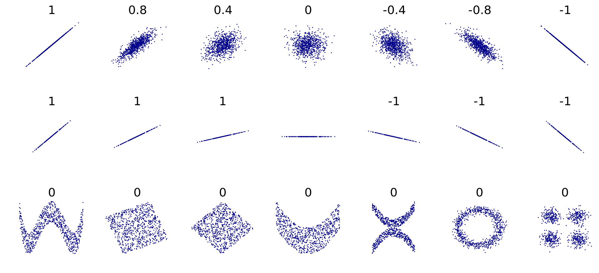
Figure 4.4: Correlations are blind on some eye

Figure 4.4 shows that correlation coefficients are limited in to explaining the relationship of two variables. For example, when the slope of a relationship is zero, the correlation coefficient becomes undefined due to the variance of \(Y\) being zero. Furthermore, Pearson’s correlation coefficient is sensitive to outliers, and all correlation coefficients are prone to sample selection biases. It is crucial to be careful when attempting to correlate two variables, particularly when one represents a part and the other represents the total. It is also worth noting that small correlation values do not necessarily indicate a lack of association between variables. For example, Pearson’s correlation coefficient can underestimates the association between variables exhibiting a quadratic relationship. Therefore, it is always advisable to examine scatterplots in conjunction with correlation analysis.
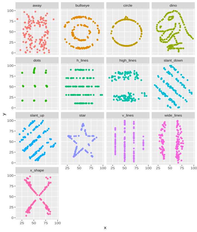
In Figure 4.5 you see various graphs that all have the same correlation coefficient and share other statistical properties like is investigated in Exercise 4.2.

Figure 4.5: These diagrams all have the same statistical properties4

4 This graph was produced employing the datasauRus R package.

4.2.2.3 Rank correlation coefficient (Spearman)

Spearman’s rank correlation coefficient is a measure of the strength and direction of the monotonic relationship between two variables. It can be calculated for a sample of size \(n\) by converting the \(n\) raw scores \(X_i, Y_i\) to ranks \(\text{R}(X_i), \text{R}(Y_i)\), then using the following formula:

\[ r_s = \rho_{\operatorname{R}(X),\operatorname{R}(Y)} = \frac{\text{cov}(\operatorname{R}(X), \operatorname{R}(Y))}{\sigma_{\operatorname{R}(X)} \sigma_{\operatorname{R}(Y)}}, \] where \(\rho\) denotes the usual Pearson correlation coefficient, but applied to the rank variables, \(\operatorname{cov}(\operatorname{R}(X), \operatorname{R}(Y))\) is the covariance of the rank variables, \(\sigma_{\operatorname{R}(X)}\) and \(\sigma_{\operatorname{R}(Y)}\) are the standard deviations of the rank variables.

If all \(n\) ranks are distinct integers, you can use the handy formula: \[ \rho = 1 - \frac{6\sum d_i^2}{n(n^2 - 1)} \] where \(\rho\) denotes the correlation coefficient, \(\sum d_i^2\) is the sum of squared differences between the ranks of corresponding pairs of variables, and \(n\) represents the number of pairs of observations.

The coefficient ranges from -1 to 1. A value of 1 indicates a perfect increasing monotonic relationship, while a value of -1 indicates a perfect decreasing monotonic relationship. A value of 0 suggests no monotonic relationship between the variables.

Spearman’s rank correlation coefficient is a non-parametric measure and is often used when the relationship between variables is not linear or when the data is in the form of ranks or ordinal categories.

Exercise 4.2 DatasauRus (Solution online.)

The following exercise shows how to create Figure 4.5 using the programming language R.

Figure 4.6: The logo of the DatasauRus package
  1. Load the packages datasauRus and tidyverse. If necessary, install these packages.

  2. The package datasauRus comes with a dataset in two different formats: datasaurus_dozen and datasaurus_dozen_wide. Store them as ds and ds_wide.

  3. Open and read the R vignette of the datasauRus package. Also open the R documentation of the dataset datasaurus_dozen.

  4. Explore the dataset: What are the dimensions of this dataset? Look at the descriptive statistics.

  5. How many unique values does the variable dataset of the tibble ds have? Hint: The function unique() return the unique values of a variable and the function length() returns the length of a vector, such as the unique elements.

  6. Compute the mean values of the x and y variables for each entry in dataset. Hint: Use the group_by() function to group the data by the appropriate column and then the summarise() function to calculate the mean.

  7. Compute the standard deviation, the correlation, and the median in the same way. Round the numbers.

  8. What can you conclude?

  9. Plot all datasets of ds. Hide the legend. Hint: Use the facet_wrap() and the theme() function.

  10. Create a loop that generates separate scatter plots for each unique datatset of the tibble ds. Export each graph as a png file.

  11. Watch the video Animating the Datasaurus Dozen Dataset in R from The Data Digest on YouTube.

Exercise 4.3 Summary statistics (Solution 4.2)

Calculate for the following datasets: the mode, the median, the 20% quantile, the range, the interquartile range, the variance, the arithmetic mean, the sample standard deviation, the coefficient of variation.

  1. For ten participants in a scientific conference the age has been noted: [25, 21, 18, 37, 56, 89, 46, 23, 21, 34.]
  2. A random sample of 128 visitors of the Cupcake festival yielded the following frequencies regarding the cupcake consumption during their visit:
Table 4.1: Random sample of 128 visitors
Cupcages consumed 1 2 3 4 5 6
Abs. freq. 2 30 37 28 23 8

Exercise 4.4 Summary statistics in spreadsheet software (Solution 4.4)

Given is the following datset: [0, 0, 40, 50, 50, 60, 70, 90, 100, 100.] Compute the following summary statistics of the data set using a spreadsheet software like or : mean, median, mode, quartiles (Q1, Q2, Q3), range, interquartile range, variance, standard deviation, mean absolute deviation, coefficient of variation and skewness.

Exercise 4.5 Guess the summary statistics (Solution 4.3)

Given are the following variables:

Table 4.2: Some variables with observations
a b c d e
97 70 1 1 970
98 80 50 2 980
99 90 50 3 990
100 100 50 4 1000
101 110 50 5 1010
102 120 50 6 1020
103 130 99 7 1030

Rank the variables without calculating concrete numbers accordingly to the values of the following descriptive statistics: mode, median, mean, range, variance, standard deviation, coefficient of variation.

Solutions to the exercises

Solution 4.1. Solution to exercise Exercise 4.1

Random sampling is a sampling procedure by which each member of a population has an equal chance of being included in the sample. Random sampling ensures a representative sample. There are several types of random sampling. In simple random sampling, not only each item in the population but each sample has an equal probability of being picked. In systematic sampling, items are selected from the population at uniform intervals of time, order, or space (as in picking every one-hundredth name from a telephone directory). Systematic sampling can be biased easily, such as, for example, when the amount of household garbage is measured on Mondays (which includes the weekend garbage). In stratified and cluster sampling, the population is divided into strata (such as age groups) and clusters (such as blocks of a city) and then a proportionate number of elements is picked at random from each stratum and cluster. Stratified sampling is used when the variations within each stratum are small in relation to the variations between strata. Cluster sampling is used when the opposite is the case. In what follows, we assume simple random sampling. Sampling can be from a finite population (as in picking cards from a deck without replacement) or from an infinite population (as in picking parts produced by a continuous process or cards from a deck with replacement). The larger the sample gets, the closer we get to the population and hence, we reduce the bias of having a non-randomly selected sample.

Solution 4.2. Solution to exercise Exercise 4.3

Metric 1 2
Mode 21 3
Median 29.5 3
P20 21 2
Range 71 5
IQR 25 1.5
Arithmetic mean 37 3.5
\(\sigma^2\) 485.33 1.5591
\(\sigma\) 22.030 1.248621
COV 0.5954 2.4027

Solution 4.3. Solution to exercise Exercise 4.5

varlabel a b c d e
Variance 2 (4.6666) 4 (466.66) 5 (800.33) 1 (4.6666) 3 (466.66)
COV 1 (.02160) 3 (.21602) 5 (.56580) 4 (.54006) 2 (.02160)
Mean 3 (100) 4 (100) 2 (50) 1 (4) 5 (1000)
Median 3 (100) 4 (100) 2 (50) 1 (4) 5 (1000)
Range 1 (6) 4 (60) 5 (98) 2 (6) 3 (60)
SD 1 (2.1602) 4 (21.602) 5 (28.290) 2 (2.1602) 3 (21.602)

Solution 4.4. Solution to exercise Exercise 4.4

Mittelwert 56
Standardfehler 11,4697670227235
Modus 0
Median 55
Erstes Quartil 42,5
Drittes Quartil 85
Varianz 1315,55555555556
Standardabweichung 36,2705880232945
Kurtosis -0,731538352420953
Schräge -0,417051115341008
Bereich 100
Minimum 0
Maximum 100
Summe 560
Anzahl 10