6 Identification
In empirical research, identification refers to the process of establishing a clear and logical relationship between a cause and an effect. This involves demonstrating that the cause is responsible for the observed effect, and that there are no other factors that could potentially explain the effect. The goal of identification is to provide strong evidence that a particular factor is indeed the cause of a particular outcome, rather than simply coincidentally happen. In order to identify a cause-and-effect relationship, researchers can use experimental or non-experimental, that is, observational data, or both. Section 5.2 will explain some difficulties researchers must face when they aim to find empirical evidence on causal effects.
6.1 Causal inference
1 Source: Cunningham (2021)

As Cunningham (2021) explains in his book (see Figure 6.1), establishing causality is very challenging. Causal inference can assist to some extent. It is the process of establishing causal relationships between variables, aiming to determine whether a change in one variable (the cause or independent variable) leads to a change in another variable (the effect or dependent variable). This process goes beyond mere association or correlation and seeks to establish that one event or factor directly influences another. Various methods of causal inference exist, and this section along with the upcoming chapters will discuss these methods. All methods share a common goal: identifying and measuring a relationship without any bias.
6.2 The fundamental problem of causal inference
Unfortunately, claiming a causal relationship to be empirically true is often not straightforward. The main reason for this lies in the so-called fundamental problem of causal inference, which is the issue of observing only one of the potential outcomes for each unit in a study. This means we lack the counterfactual outcome, which is the hypothetical outcome that would have occurred if a subject or unit had experienced a different condition or treatment than what actually happened. Thus, the fundamental problem of causal inference is actually a missing data problem.
For example, consider my son, who enjoyed throwing plates from the table. He must decide between throwing a plate or not, but he cannot do both simultaneously – an ability only possible in fictional movies like “Everything Everywhere All at Once”. Of course, my son can conduct an experiment by throwing a plate now and later deciding not to throw a plate. After observing both actions, he may claim to have found evidence that throwing a plate causes noise. However, he can never be 100% certain that the noise he heard after throwing the plate was solely caused by his action. It could be a coincidence that something else caused the noise at precisely the same time, like one of his siblings throwing a fork. He merely assumes it was due to his action. To be more certain, he might repeat the experiment hundreds of times. Even then, he can never be 100% sure. It is still not proof in a logical sense because an external factor could theoretically cause the noise. However, this is where statistics come into play: nowing the environment and the setup of his actions, it becomes extremely unlikely that the noise was not caused by his action. Knowing the setup means, we now that hasn’t been any external factor that may have caused a false a causal fallacy. As Scott Cunningham emphasizes, “prior knowledge is required in order to justify any claim about a causal finding”:
Cunningham (2021, ch. 1.3): “It is my firm belief, which I will emphasize over and over in this book, that without prior knowledge, estimated causal effects are rarely, if ever, believable. Prior knowledge is required in order to justify any claim of a causal finding. And economic theory also highlights why causal inference is necessarily a thorny task.”
To illustrate that the fundamental problem of causal inference is actually a missing data problem, let’s consider the fictitious example data presented in Table 6.1. For different individuals, dentoted as \(i\), we know whether they were received treatment \((T=1)\) or did not receive treatment \((T=0)\), as well as whether the outcome was positive \((Y=1)\) or negative \((Y=0)\). Since we do not observe the counterfactual outcomes, we are unable to determine the individual treatment effect (ITE), which is expressed as \(Y_i(1)-Y_i(0)\).
| \(i\) | \(T\) | \(Y\) | \(Y_i(1)\) | \(Y_i(0)\) | \(Y_i(1)-Y_i(0)\) |
|---|---|---|---|---|---|
| 1 | 0 | 0 | ? | 0 | ? |
| 2 | 1 | 1 | 1 | ? | ? |
| 3 | 1 | 0 | 0 | ? | ? |
| 4 | 0 | 0 | ? | 0 | ? |
| 5 | 0 | 1 | ? | 1 | ? |
6.3 Rubin causal model
If we are interested in the causal effect of a certain treatment on an outcome, we need to compare the outcome, \(Y\), of an individuals, \(i\), who received the treatment, \(1\), to the outcome, \(Y\), of the same individual, \(i\), who did not receive the treatment, \(0\):
\[ ITE_i=Y_i(1)-Y_i(0). \]
Unfortunately, as discussed in Section 6.2, this individual treatment effect (ITE) does not exist as person \(i\) can either be treated or not, but not both simultaneously. Since the counterfactual outcome is missing for each individual, we cannot observe the actual causal effect.
The Rubin model, also known as the potential outcomes framework, provides a theoretical framework for identifying causality in the context of missing data-existing.
In the model, each subject, denoted with \(i\) (for example, a person, a school), has two potential outcomes: one outcome if the subject receives the treatment (treatment condition denoted with \(T=1\)) and another outcome if the does not receive the treatment (control condition denoted with \(T=0\)). In short, the model specifies that you can use the difference of the average of a group that received the treatment and the average of the group that did not received the treatment and use it as a substitute for the ITE: \[ \mathbb{E} [\underbrace{Y_i(1)-Y_i(0)}_{ITE}] = \underbrace{\mathbb{E}[Y(1)] - \mathbb{E}[Y(0)]}_{ATE}. \tag{6.1}\]
However, the ATE is only equal to the expected ITE if certain assumptions are fulfilled. The upcoming sections will discuss these assumptions.
6.4 Its difficult to overcome the fundamental problem
Keele (2015, p. 314): “An identification analysis identifies the assumptions needed for statistical estimates to be given a causal interpretation.”
In the following we will discuss conditions that need to hold in order to empirically draw causal conclusions from the ATE without bias. This is important because equation Equation 6.1 does not necessarily hold when using observational data without a more elaborated identification strategy.
6.4.1 Example
Suppose we want to measure the effect of a vaccine on survival rates. We observed the residents of a small city with 2,000 inhabitants over the course of 30 days. On day 1, we arrived in town and injected the vaccine to 200 individuals. By day 30, we counted the deceased in both groups: four died in the vaccinated group, while eighteen died in the group of 1,800 unvaccinated individuals. With a survival rate of 98% in the vaccinated group and 99% in the unvaccinated group, it may appear that the vaccine lowers the survival rate. Imagine that study is real, would you claim that the vaccine kills because according to Equation 6.1 we could use the ATE to indicate the ITE?
The answer is yes, but only if the assumptions of ignorability (Section 6.4.2) and unconfoundedness (Section 6.4.3) are satisfied.
In brief, ignorability means that the 200 treated individuals are not systematically different from the other 1,800 individuals regarding characteristics that have an impact of the chances to survive. Considering the fact that we cannot randomly select 200 individuals from the 2,000 inhabitants due to legal constraints (as everyone has the right to choose whether or not to receive the vaccine), we must consider who is willing to get vaccinated. This selection bias may pose issues, as vulnerable populations often have a higher willingness to accept the vaccine compared to younger and healthier individuals who may fear the disease less. For example, if we vaccinated individuals with preexisting conditions that make them more vulnerable, such as the elderly or those with chronic illnesses, we cannot assume that the ATE is equal to the ITE. This is because the overall mortality risk is higher among those who received the vaccine.
Unconfoundedness means that there are no other factors that could explain both the likelihood of receiving the vaccine and the likelihood of death. For example, if vaccinated individuals were not required to stay at home during these 30 days, their likelihood of dying may increase due to greater exposure to risky situations and other people, which in turn raises their chances of contracting a disease.
Watch the video of Brady Neal’s lecture as shown in Figure 6.2. Alternatively, you can read Neal (2020, ch. 2) of his lecture notes.
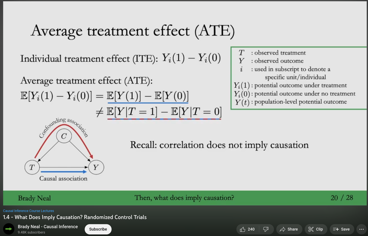
Source: Youtube
Average treatment effect (ATE)
:::
6.4.2 Ignorability
Referring to table Table 6.1, Brady Neal (2020) wrote:
“what makes it valid to calculate the ATE by taking the average of the Y(0) column, ignoring the question marks, and subtracting that from the average of the Y(1) column, ignoring the question marks?” This ignoring of the question marks (missing data) is known as ignorability. Assuming ignorability is like ignoring how people ended up selecting the treatment they selected and just assuming they were randomly assigned their treatment” (Neal, 2020, p. 9)
Ignorability means that the way individuals are assigned to treatment and control groups is irrelevant for the data analysis. Thus, when we aim to explain a certain outcome, we can ignore how an individual made it into the treated or control group. It has also been called unconfoundedness or no omitted variable bias. We will come back to these two terms in Section 7.4 and in Chapter 7.
Randomized controlled trials (RCTs) are characterized by randomly assigning individuals to different treatment groups and comparing the outcomes of those groups. Thus, RCTs are essentially build on the assumption of ignorability which can be written formally like \[ (Y(1), Y(0)) \perp T. \]
This notation indicates that the potential outcomes of an individual, \(Y\), are independent of whether they have actually received the treatment. The symbol “\(\perp\)” denotes independence, suggesting that the outcomes \(Y(1)\) and \(Y(0)\) are orthogonal to the treatment \(T\).
The assumption of ignorability allows to write the ATE as follows: \[\begin{align} \mathbb{E}[Y(1)]-\mathbb{E}[Y(0)] & =\mathbb{E}[Y(1) \mid T=1]-\mathbb{E}[Y(0) \mid T=0] \\ & =\mathbb{E}[Y \mid T=1]-\mathbb{E}[Y \mid T=0]. \end{align}\]
Another perspective on this assumption is the concept of exchangeability. Exchangeability refers to the idea that the treatment groups can be interchanged such that if they were switched, the new treatment group would have the same outcomes as the old treatment group, and the new control group would have the same outcomes as the old control group.
6.4.3 Unconfoundedness
While randomized controlled trials (RCTs) assume the concept of ignoreability, most observational data present challenges in drawing causal conclusions due to the presence of confounding factors that affect both (1) the likelihood of individuals being part of the treatment group and (2) the observed outcome. For example, regional factors can affect both the number of storks and the number of babies born in a region. These factors are typically referred to as confounders, which we discussed in Section 5.2 as having the potential to create the illusion of a causal impact where none exists. However, empirical methods are available to control for these confounders and prevent the violation of the ignoreability assumption. Formally, the assumption can be written as \[ (Y(1), Y(0)) \perp T \mid X. \] This allows to write the ATE as follows: \[\begin{align} \mathbb{E}[Y(1)\mid X]-\mathbb{E}[Y(0)\mid X] & =\mathbb{E}[Y(1) \mid T=1, X]-\mathbb{E}[Y(0) \mid T=0, X] \\ & =\mathbb{E}[Y \mid T=1, X]-\mathbb{E}[Y \mid T=0, X]. \end{align}\]
This means that we need to control for all factors (X) that influence both groups. We will revisit this topic in Section 7.4, where we will discuss the various functional impacts that must be considered to avoid causal bias.