# Install and load required libraries
# Installs 'pacman' if not already available, which is used for package management
if (!require(pacman)) install.packages("pacman")

# Unload all previously loaded packages to start fresh
suppressMessages(pacman::p_unload(all))

# Load necessary packages for data manipulation, cleaning, and visualization
pacman::p_load(
  tidyverse, # A suite of packages designed for data science that includes tools for data manipulation, plotting, and more.
  haven,     # Used for importing and exporting data with SPSS, Stata, and SAS formats.
  janitor,   # Provides functions for examining and cleaning data, such as `clean_names()` and `tabyl()`.
  WDI,       # Facilitates downloading data from the World Bank's World Development Indicators database.
  wbstats    # Provides an interface to the World Bank's APIs for a comprehensive range of data sets.
)

# Set the working directory to a project-specific folder
setwd("~/Dropbox/hsf/courses/dsr")

# Clear the current environment of any objects
rm(list = ls())5 Kickstart
Ever got a kick that actually moved you forward? Well, let’s kickstart your R adventure by walking you through a typical data analysis workflow in R, covering everything from setting up your environment to performing data analysis and visualization. Along the way, we’ll also tackle some common troubleshooting to smooth out any bumps in the road. Please don’t worry if you don’t understand some lines of code. You will learn that later on, however, you hopefully will get a sense of what it is like to work with a command line based program.
5.1 Analysing the association of weight and the price of cars
Before we start, we need to ensure that all necessary libraries are installed and loaded. We use the pacman package for convenient package management.
Now, let us load the dataset from a Stata file (auto.dta) and explore its basic properties.
# Load data from a Stata file available online
auto <- read_dta("http://www.stata-press.com/data/r18/auto.dta")
# 'auto': Dataset contains information about different car models

# Display basic information about the dataset
ncol(auto)  # Number of columns
[1] 12nrow(auto) # Number of rows[1] 74dim(auto) # Dimensions of the dataset[1] 74 12names(auto) # Names of variables [1] "make" "price" "mpg" "rep78" "headroom"
[6] "trunk" "weight" "length" "turn" "displacement"
[11] "gear_ratio" "foreign" head(auto) # First few rows# A tibble: 6 × 12
make price mpg rep78 headroom trunk weight length turn displacement
<chr> <dbl> <dbl> <dbl> <dbl> <dbl> <dbl> <dbl> <dbl> <dbl>
1 AMC Concord 4099 22 3 2.5 11 2930 186 40 121
2 AMC Pacer 4749 17 3 3 11 3350 173 40 258
3 AMC Spirit 3799 22 NA 3 12 2640 168 35 121
4 Buick Centu… 4816 20 3 4.5 16 3250 196 40 196
5 Buick Elect… 7827 15 4 4 20 4080 222 43 350
6 Buick LeSab… 5788 18 3 4 21 3670 218 43 231
# ℹ 2 more variables: gear_ratio <dbl>, foreign <dbl+lbl>tail(auto) # Last few rows# A tibble: 6 × 12
make price mpg rep78 headroom trunk weight length turn displacement
<chr> <dbl> <dbl> <dbl> <dbl> <dbl> <dbl> <dbl> <dbl> <dbl>
1 Toyota Coro… 5719 18 5 2 11 2670 175 36 134
2 VW Dasher 7140 23 4 2.5 12 2160 172 36 97
3 VW Diesel 5397 41 5 3 15 2040 155 35 90
4 VW Rabbit 4697 25 4 3 15 1930 155 35 89
5 VW Scirocco 6850 25 4 2 16 1990 156 36 97
6 Volvo 260 11995 17 5 2.5 14 3170 193 37 163
# ℹ 2 more variables: gear_ratio <dbl>, foreign <dbl+lbl>summary(auto) # Summary statistics for each column make price mpg rep78
Length:74 Min. : 3291 Min. :12.00 Min. :1.000
Class :character 1st Qu.: 4220 1st Qu.:18.00 1st Qu.:3.000
Mode :character Median : 5006 Median :20.00 Median :3.000
Mean : 6165 Mean :21.30 Mean :3.406
3rd Qu.: 6332 3rd Qu.:24.75 3rd Qu.:4.000
Max. :15906 Max. :41.00 Max. :5.000
NA's :5
headroom trunk weight length turn
Min. :1.500 Min. : 5.00 Min. :1760 Min. :142.0 Min. :31.00
1st Qu.:2.500 1st Qu.:10.25 1st Qu.:2250 1st Qu.:170.0 1st Qu.:36.00
Median :3.000 Median :14.00 Median :3190 Median :192.5 Median :40.00
Mean :2.993 Mean :13.76 Mean :3019 Mean :187.9 Mean :39.65
3rd Qu.:3.500 3rd Qu.:16.75 3rd Qu.:3600 3rd Qu.:203.8 3rd Qu.:43.00
Max. :5.000 Max. :23.00 Max. :4840 Max. :233.0 Max. :51.00
displacement gear_ratio foreign
Min. : 79.0 Min. :2.190 Min. :0.0000
1st Qu.:119.0 1st Qu.:2.730 1st Qu.:0.0000
Median :196.0 Median :2.955 Median :0.0000
Mean :197.3 Mean :3.015 Mean :0.2973
3rd Qu.:245.2 3rd Qu.:3.352 3rd Qu.:1.0000
Max. :425.0 Max. :3.890 Max. :1.0000
glimpse(auto) # Compact display of the structure of the datasetRows: 74
Columns: 12
$ make <chr> "AMC Concord", "AMC Pacer", "AMC Spirit", "Buick Century"…
$ price <dbl> 4099, 4749, 3799, 4816, 7827, 5788, 4453, 5189, 10372, 40…
$ mpg <dbl> 22, 17, 22, 20, 15, 18, 26, 20, 16, 19, 14, 14, 21, 29, 1…
$ rep78 <dbl> 3, 3, NA, 3, 4, 3, NA, 3, 3, 3, 3, 2, 3, 3, 4, 3, 2, 2, 3…
$ headroom <dbl> 2.5, 3.0, 3.0, 4.5, 4.0, 4.0, 3.0, 2.0, 3.5, 3.5, 4.0, 3.…
$ trunk <dbl> 11, 11, 12, 16, 20, 21, 10, 16, 17, 13, 20, 16, 13, 9, 20…
$ weight <dbl> 2930, 3350, 2640, 3250, 4080, 3670, 2230, 3280, 3880, 340…
$ length <dbl> 186, 173, 168, 196, 222, 218, 170, 200, 207, 200, 221, 20…
$ turn <dbl> 40, 40, 35, 40, 43, 43, 34, 42, 43, 42, 44, 43, 45, 34, 4…
$ displacement <dbl> 121, 258, 121, 196, 350, 231, 304, 196, 231, 231, 425, 35…
$ gear_ratio <dbl> 3.58, 2.53, 3.08, 2.93, 2.41, 2.73, 2.87, 2.93, 2.93, 3.0…
$ foreign <dbl+lbl> 0, 0, 0, 0, 0, 0, 0, 0, 0, 0, 0, 0, 0, 0, 0, 0, 0, 0,…print(auto, n = Inf) # Print all rows of the dataset# A tibble: 74 × 12
make price mpg rep78 headroom trunk weight length turn displacement
<chr> <dbl> <dbl> <dbl> <dbl> <dbl> <dbl> <dbl> <dbl> <dbl>
1 AMC Concord 4099 22 3 2.5 11 2930 186 40 121
2 AMC Pacer 4749 17 3 3 11 3350 173 40 258
3 AMC Spirit 3799 22 NA 3 12 2640 168 35 121
4 Buick Cent… 4816 20 3 4.5 16 3250 196 40 196
5 Buick Elec… 7827 15 4 4 20 4080 222 43 350
6 Buick LeSa… 5788 18 3 4 21 3670 218 43 231
7 Buick Opel 4453 26 NA 3 10 2230 170 34 304
8 Buick Regal 5189 20 3 2 16 3280 200 42 196
9 Buick Rivi… 10372 16 3 3.5 17 3880 207 43 231
10 Buick Skyl… 4082 19 3 3.5 13 3400 200 42 231
11 Cad. Devil… 11385 14 3 4 20 4330 221 44 425
12 Cad. Eldor… 14500 14 2 3.5 16 3900 204 43 350
13 Cad. Sevil… 15906 21 3 3 13 4290 204 45 350
14 Chev. Chev… 3299 29 3 2.5 9 2110 163 34 231
15 Chev. Impa… 5705 16 4 4 20 3690 212 43 250
16 Chev. Mali… 4504 22 3 3.5 17 3180 193 31 200
17 Chev. Mont… 5104 22 2 2 16 3220 200 41 200
18 Chev. Monza 3667 24 2 2 7 2750 179 40 151
19 Chev. Nova 3955 19 3 3.5 13 3430 197 43 250
20 Dodge Colt 3984 30 5 2 8 2120 163 35 98
21 Dodge Dipl… 4010 18 2 4 17 3600 206 46 318
22 Dodge Magn… 5886 16 2 4 17 3600 206 46 318
23 Dodge St. … 6342 17 2 4.5 21 3740 220 46 225
24 Ford Fiesta 4389 28 4 1.5 9 1800 147 33 98
25 Ford Musta… 4187 21 3 2 10 2650 179 43 140
26 Linc. Cont… 11497 12 3 3.5 22 4840 233 51 400
27 Linc. Mark… 13594 12 3 2.5 18 4720 230 48 400
28 Linc. Vers… 13466 14 3 3.5 15 3830 201 41 302
29 Merc. Bobc… 3829 22 4 3 9 2580 169 39 140
30 Merc. Coug… 5379 14 4 3.5 16 4060 221 48 302
31 Merc. Marq… 6165 15 3 3.5 23 3720 212 44 302
32 Merc. Mona… 4516 18 3 3 15 3370 198 41 250
33 Merc. XR-7 6303 14 4 3 16 4130 217 45 302
34 Merc. Zeph… 3291 20 3 3.5 17 2830 195 43 140
35 Olds 98 8814 21 4 4 20 4060 220 43 350
36 Olds Cutl … 5172 19 3 2 16 3310 198 42 231
37 Olds Cutla… 4733 19 3 4.5 16 3300 198 42 231
38 Olds Delta… 4890 18 4 4 20 3690 218 42 231
39 Olds Omega 4181 19 3 4.5 14 3370 200 43 231
40 Olds Starf… 4195 24 1 2 10 2730 180 40 151
41 Olds Toron… 10371 16 3 3.5 17 4030 206 43 350
42 Plym. Arrow 4647 28 3 2 11 3260 170 37 156
43 Plym. Champ 4425 34 5 2.5 11 1800 157 37 86
44 Plym. Hori… 4482 25 3 4 17 2200 165 36 105
45 Plym. Sapp… 6486 26 NA 1.5 8 2520 182 38 119
46 Plym. Vola… 4060 18 2 5 16 3330 201 44 225
47 Pont. Cata… 5798 18 4 4 20 3700 214 42 231
48 Pont. Fire… 4934 18 1 1.5 7 3470 198 42 231
49 Pont. Gran… 5222 19 3 2 16 3210 201 45 231
50 Pont. Le M… 4723 19 3 3.5 17 3200 199 40 231
51 Pont. Phoe… 4424 19 NA 3.5 13 3420 203 43 231
52 Pont. Sunb… 4172 24 2 2 7 2690 179 41 151
53 Audi 5000 9690 17 5 3 15 2830 189 37 131
54 Audi Fox 6295 23 3 2.5 11 2070 174 36 97
55 BMW 320i 9735 25 4 2.5 12 2650 177 34 121
56 Datsun 200 6229 23 4 1.5 6 2370 170 35 119
57 Datsun 210 4589 35 5 2 8 2020 165 32 85
58 Datsun 510 5079 24 4 2.5 8 2280 170 34 119
59 Datsun 810 8129 21 4 2.5 8 2750 184 38 146
60 Fiat Strada 4296 21 3 2.5 16 2130 161 36 105
61 Honda Acco… 5799 25 5 3 10 2240 172 36 107
62 Honda Civic 4499 28 4 2.5 5 1760 149 34 91
63 Mazda GLC 3995 30 4 3.5 11 1980 154 33 86
64 Peugeot 604 12990 14 NA 3.5 14 3420 192 38 163
65 Renault Le… 3895 26 3 3 10 1830 142 34 79
66 Subaru 3798 35 5 2.5 11 2050 164 36 97
67 Toyota Cel… 5899 18 5 2.5 14 2410 174 36 134
68 Toyota Cor… 3748 31 5 3 9 2200 165 35 97
69 Toyota Cor… 5719 18 5 2 11 2670 175 36 134
70 VW Dasher 7140 23 4 2.5 12 2160 172 36 97
71 VW Diesel 5397 41 5 3 15 2040 155 35 90
72 VW Rabbit 4697 25 4 3 15 1930 155 35 89
73 VW Scirocco 6850 25 4 2 16 1990 156 36 97
74 Volvo 260 11995 17 5 2.5 14 3170 193 37 163
# ℹ 2 more variables: gear_ratio <dbl>, foreign <dbl+lbl>The data seems to be a cross-section of cars. Let us check if the variable make identifies each line uniquely:
# Check for duplicate entries based on the 'make' variable
auto |>
  get_dupes(make)
No duplicate combinations found of: make# A tibble: 0 × 13
# ℹ 13 variables: make <chr>, dupe_count <int>, price <dbl>, mpg <dbl>,
# rep78 <dbl>, headroom <dbl>, trunk <dbl>, weight <dbl>, length <dbl>,
# turn <dbl>, displacement <dbl>, gear_ratio <dbl>, foreign <dbl+lbl>Indeed, the variable make has no duplicates. Now, let’s make and save some graphical visualizations:
# Create and display a scatter plot of car price versus weight
plot_weight_price <- ggplot(auto, aes(x = weight, y = price)) +
  geom_point()
plot_weight_price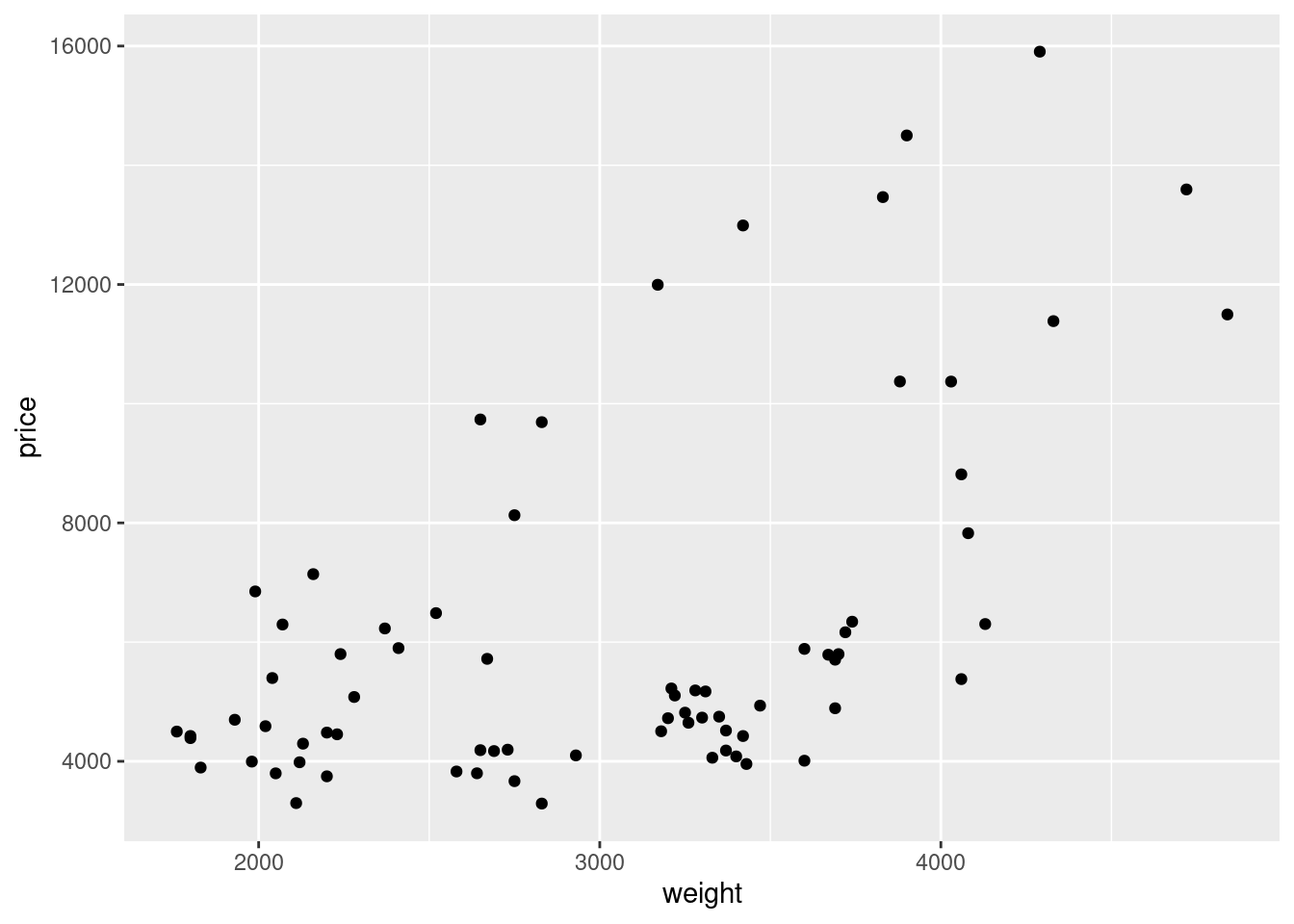
# Save the plot to a file
ggsave("fig/plot_weight_price.png", plot = plot_weight_price, dpi = 300)
Saving 7 x 5 in image# Create a scatter plot with a linear regression line of price vs weight
plot_weight_price_fit <- ggplot(auto, aes(x = weight, y = price)) +
geom_point() +
geom_smooth(method = lm, se = FALSE) # 'lm' denotes linear model, 'se' is standard error
plot_weight_price_fit`geom_smooth()` using formula = 'y ~ x'
# Save the plot to a file
ggsave("fig/plot_weight_price_fit.png", plot = plot_weight_price_fit, dpi = 300)
Saving 7 x 5 in image
`geom_smooth()` using formula = 'y ~ x'Let us perform a linear regression to quantify the impact of weight on price:
# Perform a linear regression to analyze the relationship between weight and price
reg_result <- lm(price ~ weight , data = auto)
summary(reg_result) # Display the regression results
Call:
lm(formula = price ~ weight, data = auto)

Residuals:
    Min      1Q  Median      3Q     Max
-3341.9 -1828.3  -624.1  1232.1  7143.7

Coefficients:
             Estimate Std. Error t value Pr(>|t|)
(Intercept)   -6.7074  1174.4296  -0.006    0.995
weight         2.0441     0.3768   5.424 7.42e-07 ***
---
Signif. codes:  0 '***' 0.001 '**' 0.01 '*' 0.05 '.' 0.1 ' ' 1

Residual standard error: 2502 on 72 degrees of freedom
Multiple R-squared:  0.2901,    Adjusted R-squared:  0.2802
F-statistic: 29.42 on 1 and 72 DF,  p-value: 7.416e-07
5.2 Accessing World Bank’s World Development Indicators
The World Wide Web is a treasure trove of data, and most major databases offer researchers direct download options. Numerous user-supplied packages are available for seamless access to such data. In this section, I present two popular packages that facilitate the downloading of data from the World Bank’s World Development Indicators:
WDI (World Development Indicators) Package - Official CRAN package documentation: WDI on CRAN - Source code on GitHub: WDI GitHub Repository
wbstats (World Bank Statistics) Package - Official CRAN package documentation: wbstats on CRAN - Source code on GitHub: wbstats GitHub Repository
Now, let’s download some GDP data and explore how to manipulate it. This exercise will demonstrate practical applications of the tools.
# Search for GDP indicators and display the first 10
WDIsearch("gdp")[1:10, ]
indicator name
689 6.0.GDP_current GDP (current $)
690 6.0.GDP_growth GDP growth (annual %)
691 6.0.GDP_usd GDP (constant 2005 $)
692 6.0.GDPpc_constant GDP per capita, PPP (constant 2011 international $)
2096 BG.GSR.NFSV.GD.ZS Trade in services (% of GDP)
2097 BG.KAC.FNEI.GD.PP.ZS Gross private capital flows (% of GDP, PPP)
2098 BG.KAC.FNEI.GD.ZS Gross private capital flows (% of GDP)
2099 BG.KLT.DINV.GD.PP.ZS Gross foreign direct investment (% of GDP, PPP)
2100 BG.KLT.DINV.GD.ZS Gross foreign direct investment (% of GDP)
2401 BI.WAG.TOTL.GD.ZS Wage bill as a percentage of GDP# Retrieve GDP per capita data for specified countries and years
df_WDI <- WDI(
indicator = "NY.GDP.PCAP.KD",
country = c("MX", "CA", "US"),
start = 1960,
end = 2012
)
# Plot GDP per capita over time for the specified countries
ggplot(df_WDI, aes(year, NY.GDP.PCAP.KD, color = country)) +
geom_line() +
xlab("Year") +
ylab("GDP per capita")
# Retrieve GDP per capita data for specified countries and years using the wbstats package
df_wb <- wb_data(
  indicator = "NY.GDP.PCAP.KD",
  country = c("MX", "CA", "US"),
  start = 1960,
  end = 2012,
  return_wide = TRUE
)

# Plot GDP per capita over time for the specified countries
ggplot(df_wb, aes(date, NY.GDP.PCAP.KD, color = country)) +
  geom_line() +
  xlab("Year") +
  ylab("GDP per capita (constant 2010 US$)")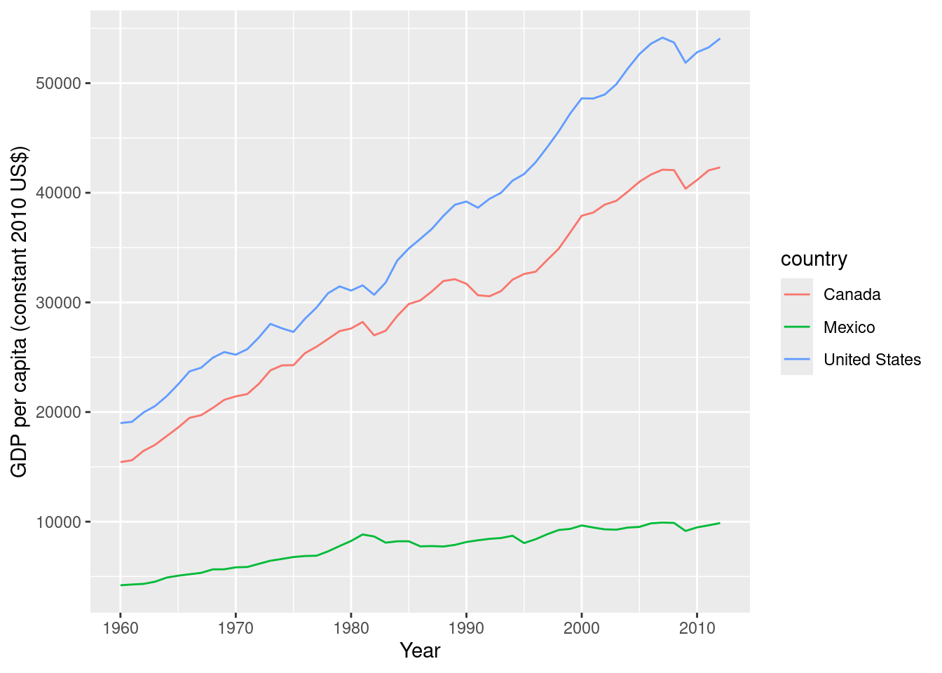
The latter graph appears empty. Why? Let’s take a closer look at the data to identify any discrepancies that might explain this issue:
# Look at the data types year and date are different:
glimpse(df_WDI)
Rows: 159
Columns: 5
$ country <chr> "Canada", "Canada", "Canada", "Canada", "Canada", "Cana…
$ iso2c <chr> "CA", "CA", "CA", "CA", "CA", "CA", "CA", "CA", "CA", "…
$ iso3c <chr> "CAN", "CAN", "CAN", "CAN", "CAN", "CAN", "CAN", "CAN",…
$ year <int> 2012, 2011, 2010, 2009, 2008, 2007, 2006, 2005, 2004, 2…
$ NY.GDP.PCAP.KD <dbl> 42320.64, 42043.64, 41164.34, 40376.42, 42067.57, 42106…glimpse(df_wb)Rows: 159
Columns: 9
$ iso2c <chr> "CA", "CA", "CA", "CA", "CA", "CA", "CA", "CA", "CA", "…
$ iso3c <chr> "CAN", "CAN", "CAN", "CAN", "CAN", "CAN", "CAN", "CAN",…
$ country <chr> "Canada", "Canada", "Canada", "Canada", "Canada", "Cana…
$ date <dbl> 1960, 1961, 1962, 1963, 1964, 1965, 1966, 1967, 1968, 1…
$ NY.GDP.PCAP.KD <dbl> 15432.47, 15605.52, 16455.75, 17007.69, 17800.86, 18585…
$ unit <chr> NA, NA, NA, NA, NA, NA, NA, NA, NA, NA, NA, NA, NA, NA,…
$ obs_status <chr> NA, NA, NA, NA, NA, NA, NA, NA, NA, NA, NA, NA, NA, NA,…
$ footnote <chr> NA, NA, NA, NA, NA, NA, NA, NA, NA, NA, NA, NA, NA, NA,…
$ last_updated <date> 2025-04-15, 2025-04-15, 2025-04-15, 2025-04-15, 2025-0…The answer is: A lineplot with a character variable (date is <chr>) on the x-axis does not work!
Now, let us manipulate the df_wb data so that the two dataset are equal:
df_wb_cln <- df_wb |>
  # Convert 'date' in df_wb from character to integer
  mutate(year = as.integer(date)) |>
  # Since 'year' has been created, remove the original 'date' column
  select(-date) |>
  # Relocate columns to organize the data frame
  relocate(country, iso2c, iso3c, year, NY.GDP.PCAP.KD)

glimpse(df_WDI)
Rows: 159
Columns: 5
$ country <chr> "Canada", "Canada", "Canada", "Canada", "Canada", "Cana…
$ iso2c <chr> "CA", "CA", "CA", "CA", "CA", "CA", "CA", "CA", "CA", "…
$ iso3c <chr> "CAN", "CAN", "CAN", "CAN", "CAN", "CAN", "CAN", "CAN",…
$ year <int> 2012, 2011, 2010, 2009, 2008, 2007, 2006, 2005, 2004, 2…
$ NY.GDP.PCAP.KD <dbl> 42320.64, 42043.64, 41164.34, 40376.42, 42067.57, 42106…glimpse(df_wb_cln)Rows: 159
Columns: 9
$ country <chr> "Canada", "Canada", "Canada", "Canada", "Canada", "Cana…
$ iso2c <chr> "CA", "CA", "CA", "CA", "CA", "CA", "CA", "CA", "CA", "…
$ iso3c <chr> "CAN", "CAN", "CAN", "CAN", "CAN", "CAN", "CAN", "CAN",…
$ year <int> 1960, 1961, 1962, 1963, 1964, 1965, 1966, 1967, 1968, 1…
$ NY.GDP.PCAP.KD <dbl> 15432.47, 15605.52, 16455.75, 17007.69, 17800.86, 18585…
$ unit <chr> NA, NA, NA, NA, NA, NA, NA, NA, NA, NA, NA, NA, NA, NA,…
$ obs_status <chr> NA, NA, NA, NA, NA, NA, NA, NA, NA, NA, NA, NA, NA, NA,…
$ footnote <chr> NA, NA, NA, NA, NA, NA, NA, NA, NA, NA, NA, NA, NA, NA,…
$ last_updated <date> 2025-04-15, 2025-04-15, 2025-04-15, 2025-04-15, 2025-0…Now it works:
# Plot GDP per capita over time for the specified countries
ggplot(df_wb_cln, aes(year, NY.GDP.PCAP.KD, color = country)) +
  geom_line() +
  xlab("Year") +
  ylab("GDP per capita (constant 2010 US$)")
Solution
The script uses the following functions: aes, as.integer, c, dim, geom_line, geom_point, geom_smooth, get_dupes, ggplot, ggsave, glimpse, head, lm, mutate, names, ncol, nrow, print, read_dta, relocate, select, setwd, summary, tail, wb, WDI, WDIsearch, xlab, ylab.
Output of the R script
# This script demonstrates a typical data analysis workflow in R
# ---------------------------------------------------------------

# Install and load required libraries
# Installs 'pacman' if not already available, which is used for package management
if (!require(pacman)) install.packages("pacman")

# Unload all previously loaded packages to start fresh
suppressMessages(pacman::p_unload(all))

# Load necessary packages for data manipulation, cleaning, and visualization
pacman::p_load(
  tidyverse, # A suite of packages designed for data science that includes tools for data manipulation, plotting, and more.
  haven, # Used for importing and exporting data with SPSS, Stata, and SAS formats.
  janitor, # Provides functions for examining and cleaning data, such as `clean_names()` and `tabyl()`.
  WDI, # Facilitates downloading data from the World Bank's World Development Indicators database.
  wbstats # Provides an interface to the World Bank's APIs for a comprehensive range of data sets.
)

# Set the working directory to a project-specific folder
setwd("~/Dropbox/hsf/courses/dsr")

# Clear the current environment of any objects
rm(list = ls())

# ---------------------------------------------------------------

# Load data from a Stata file available online
auto <- read_dta("http://www.stata-press.com/data/r8/auto.dta")
# 'auto': Dataset contains information about different car models

# Display basic information about the dataset
ncol(auto) # Number of columns
[1] 12nrow(auto) # Number of rows[1] 74dim(auto) # Dimensions of the dataset[1] 74 12names(auto) # Names of variables [1] "make" "price" "mpg" "rep78" "headroom"
[6] "trunk" "weight" "length" "turn" "displacement"
[11] "gear_ratio" "foreign" head(auto) # First few rows# A tibble: 6 × 12
make price mpg rep78 headroom trunk weight length turn displacement
<chr> <dbl> <dbl> <dbl> <dbl> <dbl> <dbl> <dbl> <dbl> <dbl>
1 AMC Concord 4099 22 3 2.5 11 2930 186 40 121
2 AMC Pacer 4749 17 3 3 11 3350 173 40 258
3 AMC Spirit 3799 22 NA 3 12 2640 168 35 121
4 Buick Centu… 4816 20 3 4.5 16 3250 196 40 196
5 Buick Elect… 7827 15 4 4 20 4080 222 43 350
6 Buick LeSab… 5788 18 3 4 21 3670 218 43 231
# ℹ 2 more variables: gear_ratio <dbl>, foreign <dbl+lbl>tail(auto) # Last few rows# A tibble: 6 × 12
make price mpg rep78 headroom trunk weight length turn displacement
<chr> <dbl> <dbl> <dbl> <dbl> <dbl> <dbl> <dbl> <dbl> <dbl>
1 Toyota Coro… 5719 18 5 2 11 2670 175 36 134
2 VW Dasher 7140 23 4 2.5 12 2160 172 36 97
3 VW Diesel 5397 41 5 3 15 2040 155 35 90
4 VW Rabbit 4697 25 4 3 15 1930 155 35 89
5 VW Scirocco 6850 25 4 2 16 1990 156 36 97
6 Volvo 260 11995 17 5 2.5 14 3170 193 37 163
# ℹ 2 more variables: gear_ratio <dbl>, foreign <dbl+lbl>summary(auto) # Summary statistics for each column make price mpg rep78
Length:74 Min. : 3291 Min. :12.00 Min. :1.000
Class :character 1st Qu.: 4220 1st Qu.:18.00 1st Qu.:3.000
Mode :character Median : 5006 Median :20.00 Median :3.000
Mean : 6165 Mean :21.30 Mean :3.406
3rd Qu.: 6332 3rd Qu.:24.75 3rd Qu.:4.000
Max. :15906 Max. :41.00 Max. :5.000
NA's :5
headroom trunk weight length turn
Min. :1.500 Min. : 5.00 Min. :1760 Min. :142.0 Min. :31.00
1st Qu.:2.500 1st Qu.:10.25 1st Qu.:2250 1st Qu.:170.0 1st Qu.:36.00
Median :3.000 Median :14.00 Median :3190 Median :192.5 Median :40.00
Mean :2.993 Mean :13.76 Mean :3019 Mean :187.9 Mean :39.65
3rd Qu.:3.500 3rd Qu.:16.75 3rd Qu.:3600 3rd Qu.:203.8 3rd Qu.:43.00
Max. :5.000 Max. :23.00 Max. :4840 Max. :233.0 Max. :51.00
displacement gear_ratio foreign
Min. : 79.0 Min. :2.190 Min. :0.0000
1st Qu.:119.0 1st Qu.:2.730 1st Qu.:0.0000
Median :196.0 Median :2.955 Median :0.0000
Mean :197.3 Mean :3.015 Mean :0.2973
3rd Qu.:245.2 3rd Qu.:3.352 3rd Qu.:1.0000
Max. :425.0 Max. :3.890 Max. :1.0000
glimpse(auto) # Compact display of the structure of the datasetRows: 74
Columns: 12
$ make <chr> "AMC Concord", "AMC Pacer", "AMC Spirit", "Buick Century"…
$ price <dbl> 4099, 4749, 3799, 4816, 7827, 5788, 4453, 5189, 10372, 40…
$ mpg <dbl> 22, 17, 22, 20, 15, 18, 26, 20, 16, 19, 14, 14, 21, 29, 1…
$ rep78 <dbl> 3, 3, NA, 3, 4, 3, NA, 3, 3, 3, 3, 2, 3, 3, 4, 3, 2, 2, 3…
$ headroom <dbl> 2.5, 3.0, 3.0, 4.5, 4.0, 4.0, 3.0, 2.0, 3.5, 3.5, 4.0, 3.…
$ trunk <dbl> 11, 11, 12, 16, 20, 21, 10, 16, 17, 13, 20, 16, 13, 9, 20…
$ weight <dbl> 2930, 3350, 2640, 3250, 4080, 3670, 2230, 3280, 3880, 340…
$ length <dbl> 186, 173, 168, 196, 222, 218, 170, 200, 207, 200, 221, 20…
$ turn <dbl> 40, 40, 35, 40, 43, 43, 34, 42, 43, 42, 44, 43, 45, 34, 4…
$ displacement <dbl> 121, 258, 121, 196, 350, 231, 304, 196, 231, 231, 425, 35…
$ gear_ratio <dbl> 3.58, 2.53, 3.08, 2.93, 2.41, 2.73, 2.87, 2.93, 2.93, 3.0…
$ foreign <dbl+lbl> 0, 0, 0, 0, 0, 0, 0, 0, 0, 0, 0, 0, 0, 0, 0, 0, 0, 0,…print(auto, n = Inf) # Print all rows of the dataset# A tibble: 74 × 12
make price mpg rep78 headroom trunk weight length turn displacement
<chr> <dbl> <dbl> <dbl> <dbl> <dbl> <dbl> <dbl> <dbl> <dbl>
1 AMC Concord 4099 22 3 2.5 11 2930 186 40 121
2 AMC Pacer 4749 17 3 3 11 3350 173 40 258
3 AMC Spirit 3799 22 NA 3 12 2640 168 35 121
4 Buick Cent… 4816 20 3 4.5 16 3250 196 40 196
5 Buick Elec… 7827 15 4 4 20 4080 222 43 350
6 Buick LeSa… 5788 18 3 4 21 3670 218 43 231
7 Buick Opel 4453 26 NA 3 10 2230 170 34 304
8 Buick Regal 5189 20 3 2 16 3280 200 42 196
9 Buick Rivi… 10372 16 3 3.5 17 3880 207 43 231
10 Buick Skyl… 4082 19 3 3.5 13 3400 200 42 231
11 Cad. Devil… 11385 14 3 4 20 4330 221 44 425
12 Cad. Eldor… 14500 14 2 3.5 16 3900 204 43 350
13 Cad. Sevil… 15906 21 3 3 13 4290 204 45 350
14 Chev. Chev… 3299 29 3 2.5 9 2110 163 34 231
15 Chev. Impa… 5705 16 4 4 20 3690 212 43 250
16 Chev. Mali… 4504 22 3 3.5 17 3180 193 31 200
17 Chev. Mont… 5104 22 2 2 16 3220 200 41 200
18 Chev. Monza 3667 24 2 2 7 2750 179 40 151
19 Chev. Nova 3955 19 3 3.5 13 3430 197 43 250
20 Dodge Colt 3984 30 5 2 8 2120 163 35 98
21 Dodge Dipl… 4010 18 2 4 17 3600 206 46 318
22 Dodge Magn… 5886 16 2 4 17 3600 206 46 318
23 Dodge St. … 6342 17 2 4.5 21 3740 220 46 225
24 Ford Fiesta 4389 28 4 1.5 9 1800 147 33 98
25 Ford Musta… 4187 21 3 2 10 2650 179 43 140
26 Linc. Cont… 11497 12 3 3.5 22 4840 233 51 400
27 Linc. Mark… 13594 12 3 2.5 18 4720 230 48 400
28 Linc. Vers… 13466 14 3 3.5 15 3830 201 41 302
29 Merc. Bobc… 3829 22 4 3 9 2580 169 39 140
30 Merc. Coug… 5379 14 4 3.5 16 4060 221 48 302
31 Merc. Marq… 6165 15 3 3.5 23 3720 212 44 302
32 Merc. Mona… 4516 18 3 3 15 3370 198 41 250
33 Merc. XR-7 6303 14 4 3 16 4130 217 45 302
34 Merc. Zeph… 3291 20 3 3.5 17 2830 195 43 140
35 Olds 98 8814 21 4 4 20 4060 220 43 350
36 Olds Cutl … 5172 19 3 2 16 3310 198 42 231
37 Olds Cutla… 4733 19 3 4.5 16 3300 198 42 231
38 Olds Delta… 4890 18 4 4 20 3690 218 42 231
39 Olds Omega 4181 19 3 4.5 14 3370 200 43 231
40 Olds Starf… 4195 24 1 2 10 2730 180 40 151
41 Olds Toron… 10371 16 3 3.5 17 4030 206 43 350
42 Plym. Arrow 4647 28 3 2 11 3260 170 37 156
43 Plym. Champ 4425 34 5 2.5 11 1800 157 37 86
44 Plym. Hori… 4482 25 3 4 17 2200 165 36 105
45 Plym. Sapp… 6486 26 NA 1.5 8 2520 182 38 119
46 Plym. Vola… 4060 18 2 5 16 3330 201 44 225
47 Pont. Cata… 5798 18 4 4 20 3700 214 42 231
48 Pont. Fire… 4934 18 1 1.5 7 3470 198 42 231
49 Pont. Gran… 5222 19 3 2 16 3210 201 45 231
50 Pont. Le M… 4723 19 3 3.5 17 3200 199 40 231
51 Pont. Phoe… 4424 19 NA 3.5 13 3420 203 43 231
52 Pont. Sunb… 4172 24 2 2 7 2690 179 41 151
53 Audi 5000 9690 17 5 3 15 2830 189 37 131
54 Audi Fox 6295 23 3 2.5 11 2070 174 36 97
55 BMW 320i 9735 25 4 2.5 12 2650 177 34 121
56 Datsun 200 6229 23 4 1.5 6 2370 170 35 119
57 Datsun 210 4589 35 5 2 8 2020 165 32 85
58 Datsun 510 5079 24 4 2.5 8 2280 170 34 119
59 Datsun 810 8129 21 4 2.5 8 2750 184 38 146
60 Fiat Strada 4296 21 3 2.5 16 2130 161 36 105
61 Honda Acco… 5799 25 5 3 10 2240 172 36 107
62 Honda Civic 4499 28 4 2.5 5 1760 149 34 91
63 Mazda GLC 3995 30 4 3.5 11 1980 154 33 86
64 Peugeot 604 12990 14 NA 3.5 14 3420 192 38 163
65 Renault Le… 3895 26 3 3 10 1830 142 34 79
66 Subaru 3798 35 5 2.5 11 2050 164 36 97
67 Toyota Cel… 5899 18 5 2.5 14 2410 174 36 134
68 Toyota Cor… 3748 31 5 3 9 2200 165 35 97
69 Toyota Cor… 5719 18 5 2 11 2670 175 36 134
70 VW Dasher 7140 23 4 2.5 12 2160 172 36 97
71 VW Diesel 5397 41 5 3 15 2040 155 35 90
72 VW Rabbit 4697 25 4 3 15 1930 155 35 89
73 VW Scirocco 6850 25 4 2 16 1990 156 36 97
74 Volvo 260 11995 17 5 2.5 14 3170 193 37 163
# ℹ 2 more variables: gear_ratio <dbl>, foreign <dbl+lbl># Check for duplicate entries based on the 'make' variable
auto |>
get_dupes(make)No duplicate combinations found of: make# A tibble: 0 × 13
# ℹ 13 variables: make <chr>, dupe_count <int>, price <dbl>, mpg <dbl>,
# rep78 <dbl>, headroom <dbl>, trunk <dbl>, weight <dbl>, length <dbl>,
# turn <dbl>, displacement <dbl>, gear_ratio <dbl>, foreign <dbl+lbl># Create and display a scatter plot of car price versus weight
plot_weight_price <- ggplot(auto, aes(x = weight, y = price)) +
geom_point()
plot_weight_price
# Save the plot to a file
ggsave("fig/plot_weight_price.png", plot = plot_weight_price, dpi = 300)
Saving 7 x 5 in image# Create a scatter plot with a linear regression line of price vs weight
plot_weight_price_fit <- ggplot(auto, aes(x = weight, y = price)) +
geom_point() +
geom_smooth(method = lm, se = FALSE) # 'lm' denotes linear model, 'se' is standard error
plot_weight_price_fit`geom_smooth()` using formula = 'y ~ x'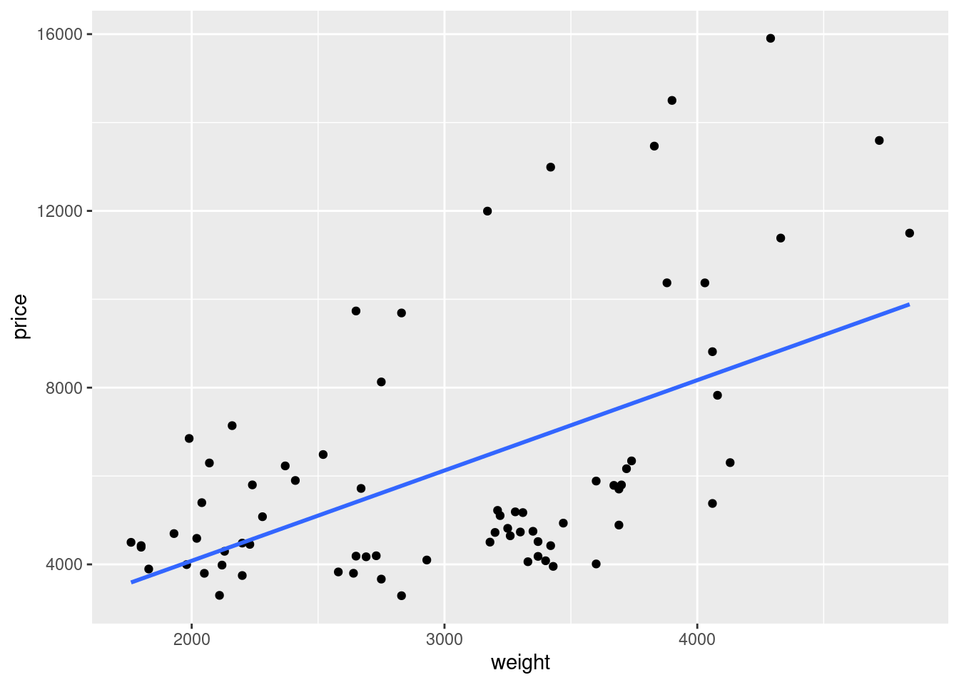
# Save the plot to a file
ggsave("fig/plot_weight_price_fit.png", plot = plot_weight_price_fit, dpi = 300)
Saving 7 x 5 in image`geom_smooth()` using formula = 'y ~ x'# Perform a linear regression to analyze the relationship between weight and price
reg_result <- lm(price ~ weight, data = auto)
summary(reg_result) # Display the regression results
Call:
lm(formula = price ~ weight, data = auto)

Residuals:
    Min      1Q  Median      3Q     Max
-3341.9 -1828.3  -624.1  1232.1  7143.7

Coefficients:
             Estimate Std. Error t value Pr(>|t|)
(Intercept)   -6.7074  1174.4296  -0.006    0.995
weight         2.0441     0.3768   5.424 7.42e-07 ***
---
Signif. codes:  0 '***' 0.001 '**' 0.01 '*' 0.05 '.' 0.1 ' ' 1

Residual standard error: 2502 on 72 degrees of freedom
Multiple R-squared:  0.2901,    Adjusted R-squared:  0.2802
F-statistic: 29.42 on 1 and 72 DF,  p-value: 7.416e-07
# Load and demonstrate usage of World Development Indicators (WDI) data
# Two different packages can help here:
# WDI:
# --- https://cran.r-project.org/web/packages/WDI/WDI.pdf
# --- https://github.com/vincentarelbundock/WDI
# wbstats:
# --- https://cran.r-project.org/web/packages/wbstats/wbstats.pdf
# --- https://github.com/gshs-ornl/wbstats
# ?WDI # Access documentation for the WDI package
# ?wbstats # # Access documentation for the wbstats package
# Search for GDP indicators and display the first 10
WDIsearch("gdp")[1:10, ] indicator name
689 6.0.GDP_current GDP (current $)
690 6.0.GDP_growth GDP growth (annual %)
691 6.0.GDP_usd GDP (constant 2005 $)
692 6.0.GDPpc_constant GDP per capita, PPP (constant 2011 international $)
2096 BG.GSR.NFSV.GD.ZS Trade in services (% of GDP)
2097 BG.KAC.FNEI.GD.PP.ZS Gross private capital flows (% of GDP, PPP)
2098 BG.KAC.FNEI.GD.ZS Gross private capital flows (% of GDP)
2099 BG.KLT.DINV.GD.PP.ZS Gross foreign direct investment (% of GDP, PPP)
2100 BG.KLT.DINV.GD.ZS Gross foreign direct investment (% of GDP)
2401 BI.WAG.TOTL.GD.ZS Wage bill as a percentage of GDP# Retrieve GDP per capita data for specified countries and years
df_WDI <- WDI(
indicator = "NY.GDP.PCAP.KD",
country = c("MX", "CA", "US"),
start = 1960,
end = 2012
)
# Plot GDP per capita over time for the specified countries
ggplot(df_WDI, aes(year, NY.GDP.PCAP.KD, color = country)) +
geom_line() +
xlab("Year") +
ylab("GDP per capita")
# Retrieve GDP per capita data for specified countries and years using the wbstats package
df_wb <- wb(
  indicator = "NY.GDP.PCAP.KD",
  country = c("MX", "CA", "US"),
  start = 1960,
  end = 2012,
  return_wide = TRUE
)
Warning: `wb()` was deprecated in wbstats 1.0.0.
ℹ Please use `wb_data()` instead.Warning: `spread_()` was deprecated in tidyr 1.2.0.
ℹ Please use `spread()` instead.
ℹ The deprecated feature was likely used in the wbstats package.
Please report the issue at <https://github.com/nset-ornl/wbstats/issues>.# Plot GDP per capita over time for the specified countries
ggplot(df_wb, aes(date, NY.GDP.PCAP.KD, color = country)) +
geom_line() +
xlab("Year") +
ylab("GDP per capita (constant 2010 US$)")`geom_line()`: Each group consists of only one observation.
ℹ Do you need to adjust the group aesthetic?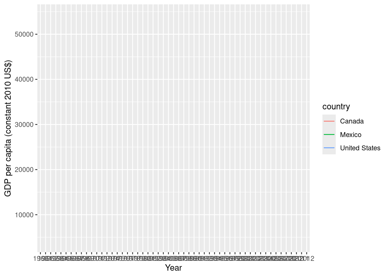
# !!! This does not work !!!
# Why?

# Look at the data types year and date are different:
glimpse(df_WDI)
Rows: 159
Columns: 5
$ country <chr> "Canada", "Canada", "Canada", "Canada", "Canada", "Cana…
$ iso2c <chr> "CA", "CA", "CA", "CA", "CA", "CA", "CA", "CA", "CA", "…
$ iso3c <chr> "CAN", "CAN", "CAN", "CAN", "CAN", "CAN", "CAN", "CAN",…
$ year <int> 2012, 2011, 2010, 2009, 2008, 2007, 2006, 2005, 2004, 2…
$ NY.GDP.PCAP.KD <dbl> 42320.64, 42043.64, 41164.34, 40376.42, 42067.57, 42106…glimpse(df_wb)Rows: 159
Columns: 5
$ iso3c <chr> "CAN", "CAN", "CAN", "CAN", "CAN", "CAN", "CAN", "CAN",…
$ date <chr> "1960", "1961", "1962", "1963", "1964", "1965", "1966",…
$ iso2c <chr> "CA", "CA", "CA", "CA", "CA", "CA", "CA", "CA", "CA", "…
$ country <chr> "Canada", "Canada", "Canada", "Canada", "Canada", "Cana…
$ NY.GDP.PCAP.KD <dbl> 15432.47, 15605.52, 16455.75, 17007.69, 17800.86, 18585…# Answer: A lineplot with a character variable on the x-axis does not work!
# make the two dataframe equal:
df_wb_cln <- df_wb |>
# Convert 'date' in df_wb from character to integer
mutate(year = as.integer(date)) |>
# Since 'year' has been created, remove the original 'date' column
select(-date) |>
# Relocate columns to organize the data frame
relocate(country, iso2c, iso3c, year, NY.GDP.PCAP.KD)
glimpse(df_WDI)Rows: 159
Columns: 5
$ country <chr> "Canada", "Canada", "Canada", "Canada", "Canada", "Cana…
$ iso2c <chr> "CA", "CA", "CA", "CA", "CA", "CA", "CA", "CA", "CA", "…
$ iso3c <chr> "CAN", "CAN", "CAN", "CAN", "CAN", "CAN", "CAN", "CAN",…
$ year <int> 2012, 2011, 2010, 2009, 2008, 2007, 2006, 2005, 2004, 2…
$ NY.GDP.PCAP.KD <dbl> 42320.64, 42043.64, 41164.34, 40376.42, 42067.57, 42106…glimpse(df_wb_cln)Rows: 159
Columns: 5
$ country <chr> "Canada", "Canada", "Canada", "Canada", "Canada", "Cana…
$ iso2c <chr> "CA", "CA", "CA", "CA", "CA", "CA", "CA", "CA", "CA", "…
$ iso3c <chr> "CAN", "CAN", "CAN", "CAN", "CAN", "CAN", "CAN", "CAN",…
$ year <int> 1960, 1961, 1962, 1963, 1964, 1965, 1966, 1967, 1968, 1…
$ NY.GDP.PCAP.KD <dbl> 15432.47, 15605.52, 16455.75, 17007.69, 17800.86, 18585…# Now it works:
# Plot GDP per capita over time for the specified countries
ggplot(df_wb_cln, aes(year, NY.GDP.PCAP.KD, color = country)) +
geom_line() +
xlab("Year") +
ylab("GDP per capita (constant 2010 US$)")
suppressMessages(pacman::p_unload(
  tidyverse, # A suite of packages designed for data science that includes tools for data manipulation, plotting, and more.
  haven, # Used for importing and exporting data with SPSS, Stata, and SAS formats.
  janitor, # Provides functions for examining and cleaning data, such as `clean_names()` and `tabyl()`.
  WDI, # Facilitates downloading data from the World Bank's World Development Indicators database.
  wbstats # Provides an interface to the World Bank's APIs for a comprehensive range of data sets.
))