The script uses among others the following functions: filter, is.na, select.
9.3 Base R,%in% operator, and the pipe |>
Using the mtcars dataset, write code to create a new dataframe that includes only the rows where the number of cylinders is either 4 or 6, and the weight (wt) is less than 3.5.
Do this in two different ways using:
The %in% operator and the pipe |> .
Base R without the pipe |>.
Compare the resulting dataframes using the identical() function.
Using the mtcars dataset, generate a logical variable that indicates with TRUE all cars with either 4 or 6 cylinders that wt is less than 3.5 and add this variable to a new dataset.
Solution
The script uses the following functions: c, filter, identical, if_else, mutate, subset, transform, with.
R script
# Base R or pipe# exe_base_pipe.R# Stephan Huber; 2023-05-08# setwd("/home/sthu/Dropbox/hsf/test")rm(list=ls())# load packagesif (!require(pacman)) install.packages("pacman")pacman::p_load(datasets, tidyverse)# a)# Using the pipe |> # Select rows where cyl is 4 or 6 and wt is less than 3.5df1 <- mtcars |>filter(cyl %in%c(4, 6) & wt <3.5) df1# Without the pipe |> # Select rows where cyl is 4 or 6 and wt is less than 3.5df2 <-subset(mtcars, cyl %in%c(4, 6) & wt <3.5)df2# Check if the resulting dataframe is identical to the expected outputidentical(df1, df2)# b)# Using the pipe |> and tidyverse (mutate)df3 <- mtcars |>mutate(cyl_4_or_6 =if_else(cyl %in%c(4, 6) & wt <3.5, TRUE, FALSE))df3# without pipe and with base R (transform)df4 <- mtcarsdf4$cyl_4_or_6 <-with(mtcars, cyl %in%c(4, 6) & wt <3.5)# Alternatively in one line:df5 <-transform(mtcars, cyl_4_or_6 = cyl %in%c(4,6) & wt <3.5)# Check if the resulting dataframe is identical to the expected outputidentical(df3, df4)identical(df3, df5)# unload packagessuppressMessages(pacman::p_unload(datasets, tidyverse))
Output of the R script
# Base R or pipe# exe_base_pipe.R# Stephan Huber; 2023-05-08# setwd("/home/sthu/Dropbox/hsf/test")rm(list=ls())# load packagesif (!require(pacman)) install.packages("pacman")pacman::p_load(datasets, tidyverse)# a)# Using the pipe |> # Select rows where cyl is 4 or 6 and wt is less than 3.5df1 <- mtcars |>filter(cyl %in%c(4, 6) & wt <3.5) df1
# without pipe and with base R (transform)df4 <- mtcarsdf4$cyl_4_or_6 <-with(mtcars, cyl %in%c(4, 6) & wt <3.5)# Alternatively in one line:df5 <-transform(mtcars, cyl_4_or_6 = cyl %in%c(4,6) & wt <3.5)# Check if the resulting dataframe is identical to the expected outputidentical(df3, df4)
Use the mtcars dataset. It is part of the package datasets and can be called with
mtcars
Create a new tibble called mtcars_new using the pipe operator |>. Generate a new dummy variable called d_cyl_6to8 that takes the value 1 if the number of cylinders (cyl) is greater than 6, and 0 otherwise. Do all of this in a single pipe.
Generate a new dummy variable called posercar that takes a value of 1 if a car has more than 6 cylinders (cyl) and can drive less than 18 miles per gallon (mpg), and 0 otherwise. Add this variable to the tibble mtcars_new.
Remove the variable d_cyl_6to8 from the data frame.
Solution
The script uses the following functions: as_tibble, if_else, mutate, rownames_to_column, select.
Check to see if you have the mtcars dataset by entering mtcars.
Save the mtcars dataset in an object named cars.
What class is cars?
How many observations (rows) and variables (columns) are in the mtcars dataset?
Rename mpg in cars to MPG. Use rename().
Convert the column names of cars to all upper case. Use rename_all, and the toupper function.
Convert the rownames of cars to a column called car using rownames_to_column.
Subset the columns from cars that end in “p” and call it pvars using ends_with().
Create a subset cars that only contains the columns: wt, qsec, and hp and assign this object to carsSub. (Use select().)
What are the dimensions of carsSub? (Use dim().)
Convert the column names of carsSub to all upper case. Use rename_all(), and toupper() (or colnames()).
Subset the rows of cars that get more than 20 miles per gallon (mpg) of fuel efficiency. How many are there? (Use filter().)
Subset the rows that get less than 16 miles per gallon (mpg) of fuel efficiency and have more than 100 horsepower (hp). How many are there? (Use filter() and the pipe operator.)
Create a subset of the cars data that only contains the columns: wt, qsec, and hp for cars with 8 cylinders (cyl) and reassign this object to carsSub. What are the dimensions of this dataset? Do not use the pipe operator.
Create a subset of the cars data that only contains the columns: wt, qsec, and hp for cars with 8 cylinders (cyl) and reassign this object to carsSub2. Use the pipe operator.
Re-order the rows of carsSub by weight (wt) in increasing order. (Use arrange().)
Create a new variable in carsSub called wt2, which is equal to wt\(^2\), using mutate() and piping |>.
Solution
The script uses the following functions: arrange, class, dim, ends_with, filter, mutate, ncol, nrow, rename, rename_all, rownames_to_column, select.
R script
# Subsetting with \R# exe_subset.R# Stephan Huber; 2022-06-07# setwd("/home/sthu/Dropbox/hsf/22-ss/dsda/work/")rm(list =ls())# 0# load packagesif (!require(pacman)) install.packages("pacman")pacman::p_load(tidyverse, dplyr, tibble)# 1mtcars# 2cars <- mtcars# 3class(cars)# 4dim(cars)# Alternativencol(cars)nrow(cars)# 5cars <-rename(cars, MPG = mpg)# 6cars <-rename_all(cars, toupper)# if you like lower cases:# cars <- rename_all(cars, tolower)# 7cars <-rownames_to_column(mtcars, var ="car")# 8pvars <-select(cars, car, ends_with("p"))# 9carsSub <-select(cars, car, wt, qsec, hp)# 10dim(carsSub)# 11carsSub <-rename_all(carsSub, toupper)# 12cars_mpg <-filter(cars, mpg >20)dim(cars_mpg)# 13cars_whattever <-filter(cars, mpg <16& hp >100)# 14carsSub <-filter(cars, cyl ==8)carsSub <-select(carsSub, wt, qsec, hp, car)dim(carsSub)# 15# Alternative with pipe operator:carsSub <- cars |>filter(cyl ==8) |>select(wt, qsec, hp, car)# 16carsSub <-arrange(carsSub, wt)# 17carsSub <- carsSub |>mutate(wt2 = wt^2)# Alternatively you can put everything into one pipe:carsSub2 <- cars |>filter(cyl ==8) |>select(wt, qsec, hp, car) |>arrange(carsSub, wt) |>mutate(wt2 = wt^2)# unload packagessuppressMessages(pacman::p_unload(tidyverse, dplyr, tibble))
Output of the R script
# Subsetting with \R# exe_subset.R# Stephan Huber; 2022-06-07# setwd("/home/sthu/Dropbox/hsf/22-ss/dsda/work/")rm(list =ls())# 0# load packagesif (!require(pacman)) install.packages("pacman")pacman::p_load(tidyverse, dplyr, tibble)# 1mtcars
Add variable mispercent that measures the percentage of missings and a variable mis30up that is 1 if the percentage is above 30%. (Hint: Use mutate, select, ifelse, and bind_cols.)
You should always try to use most recent data and you should not work outside of R. Thus, it would be optimal to download the data directly from FRED and using a R package. If this would be serious research, I would not recommend to use the data that I have downloaded from FRED, I’d recommend to use the fredr package which allows to fetch the observation directly from FRED database using the function fredr.
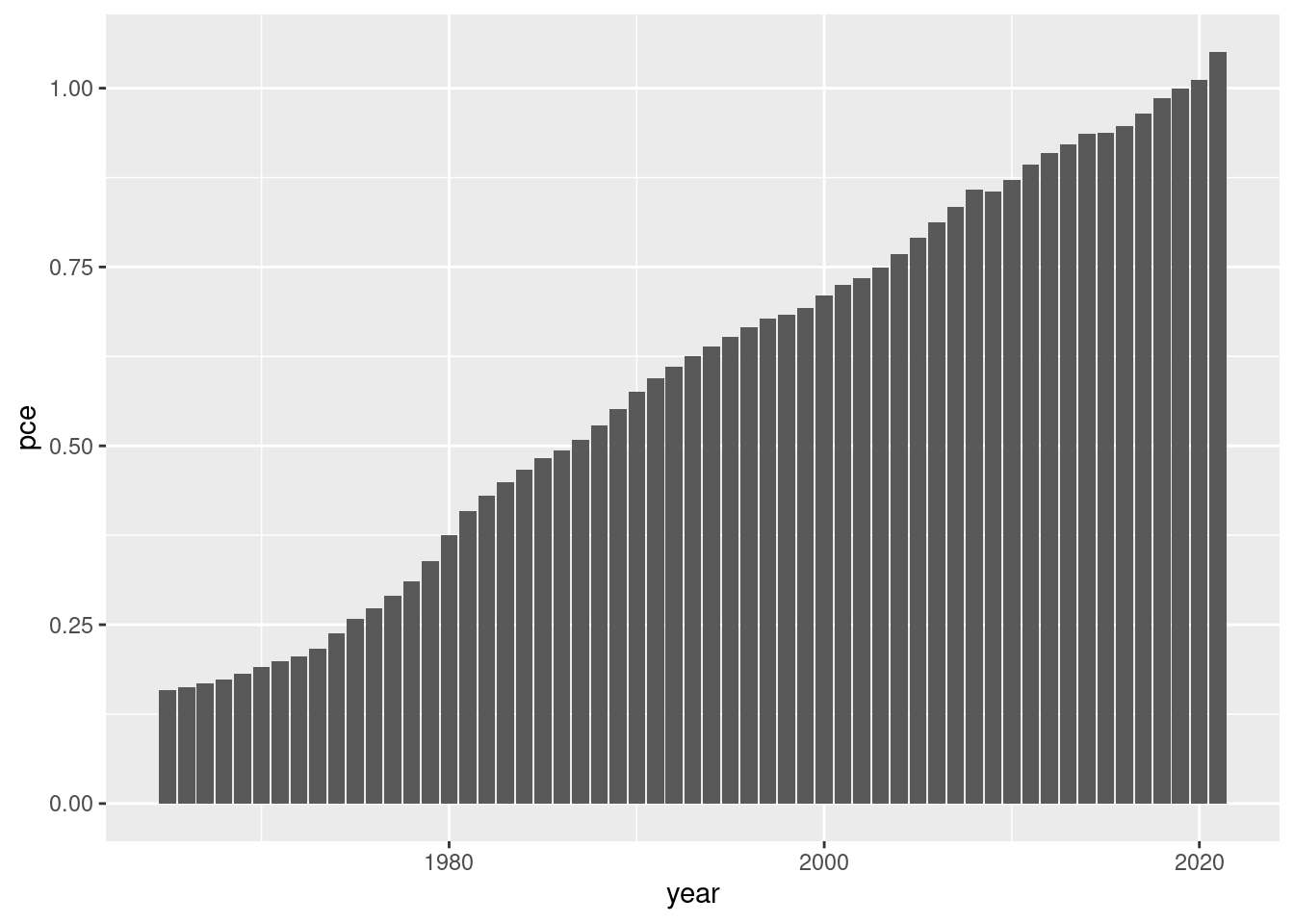
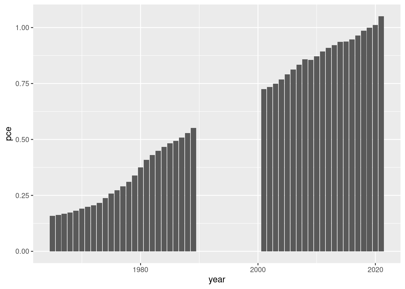
Divide the variable PCEPI_NBD20190101 by 100 and name the resulting variable pce. Additionally, generate a new variable year that contains the respective year. Save the modified dataframe as pce_cl.
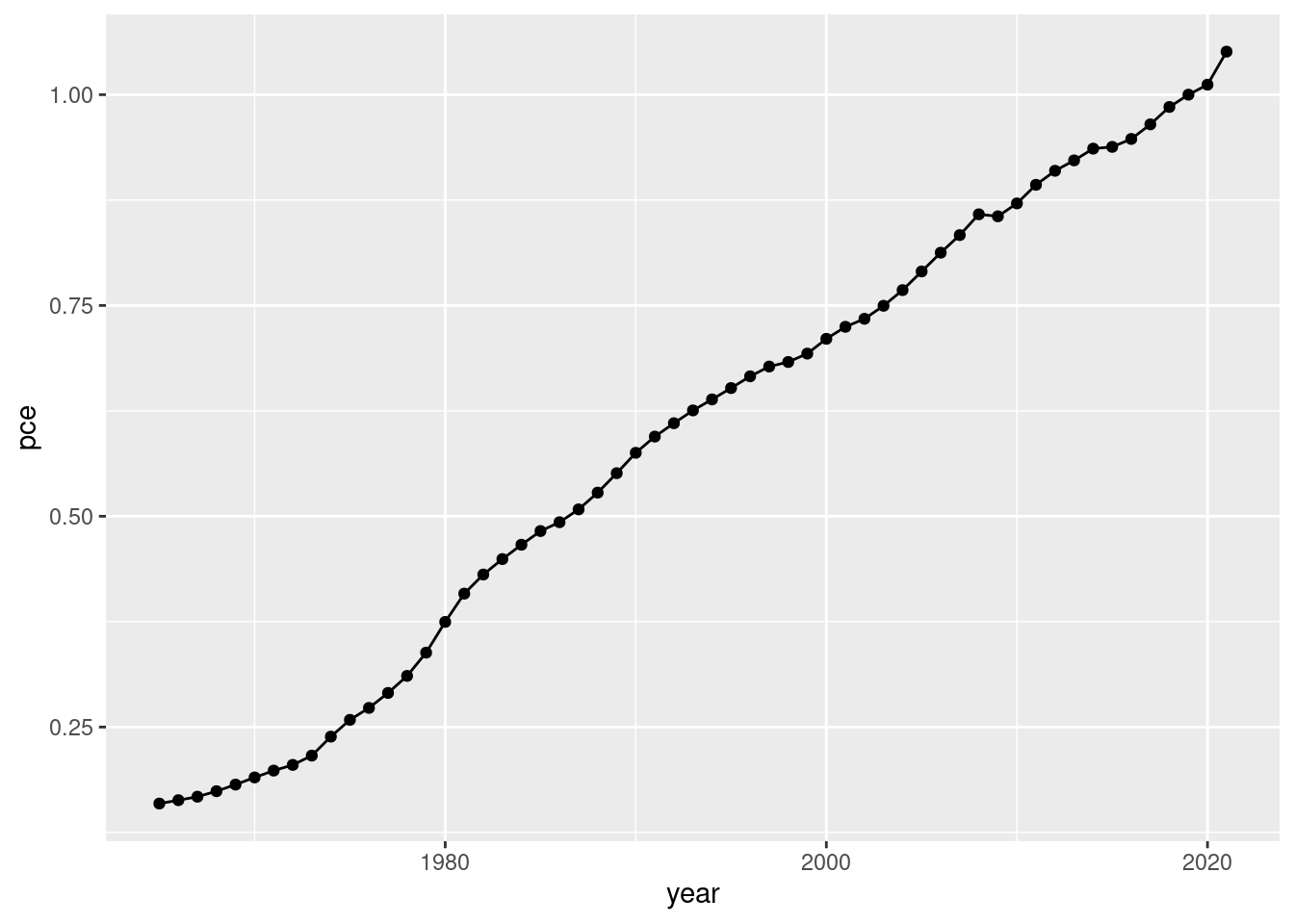
Make the following plot:
Make the following plot:
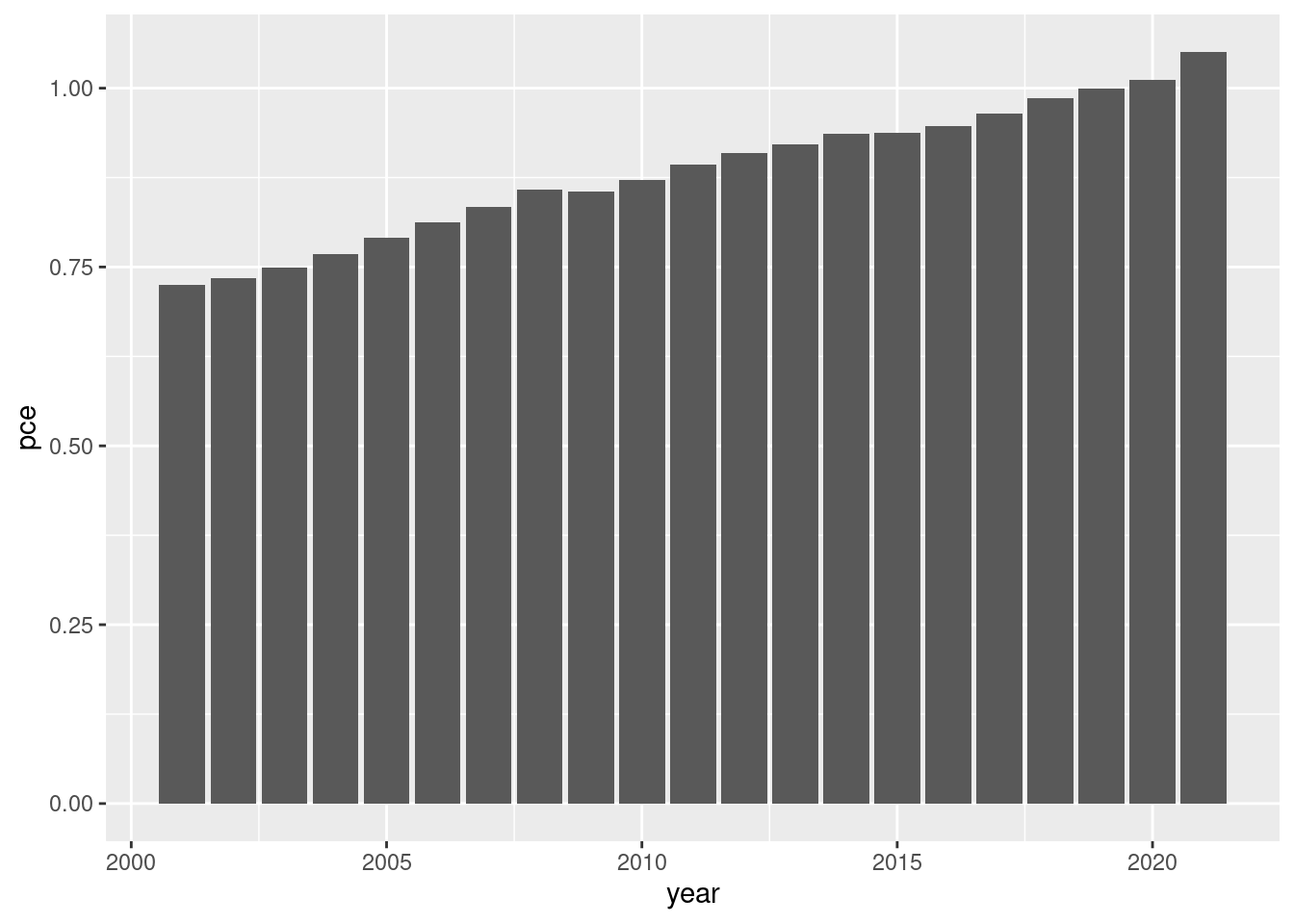
Make the following plot:
Make a plot of inflation for all years except the 90s:
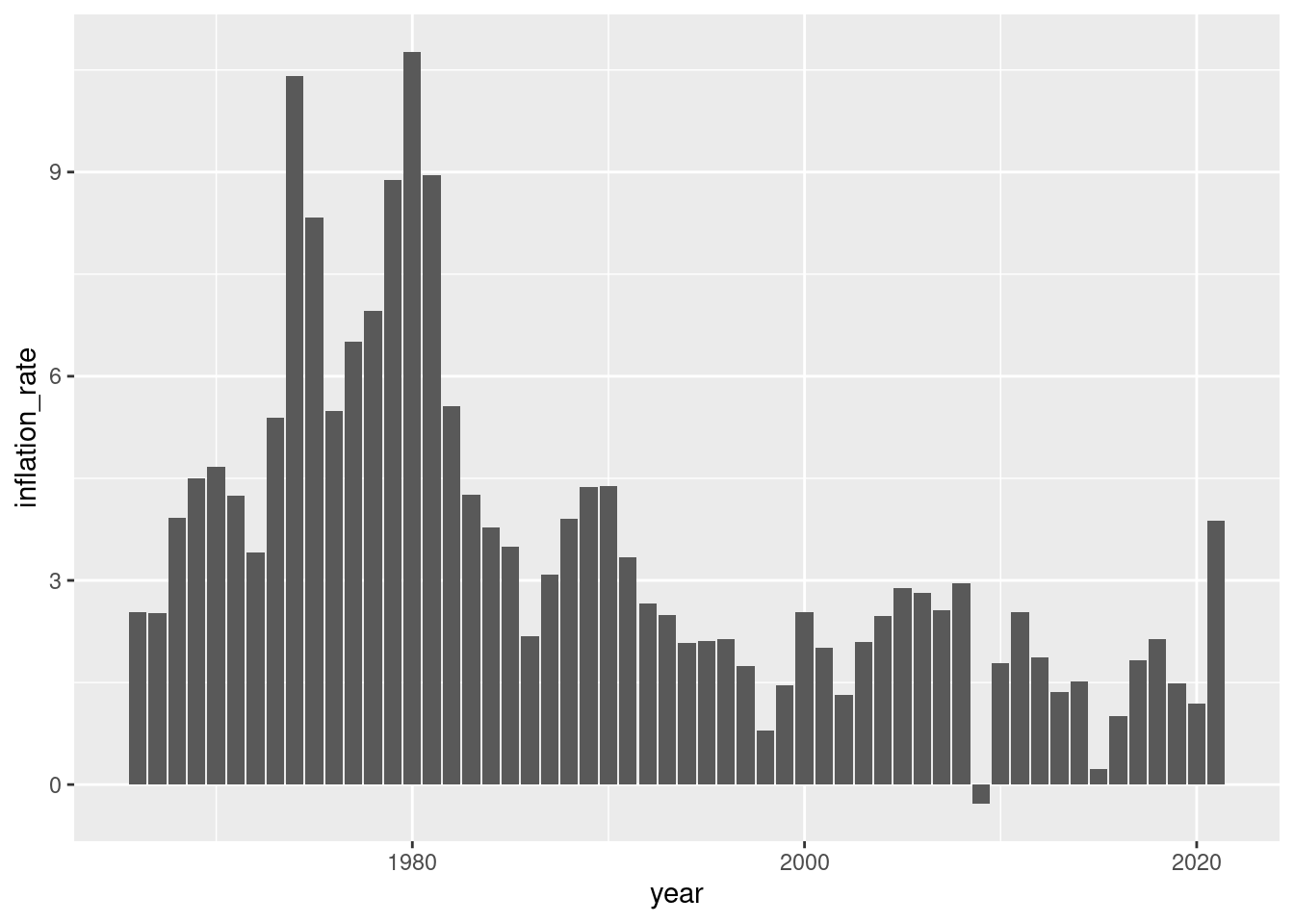
Calculate the yearly inflation. Here is an excpert of how the data should look like:
The script uses the following functions: aes, as.integer, case_when, filter, geom_bar, geom_line, geom_point, ggplot, group_by, lag, mean, mutate, read.csv, select, str_sub, summarize.
R script
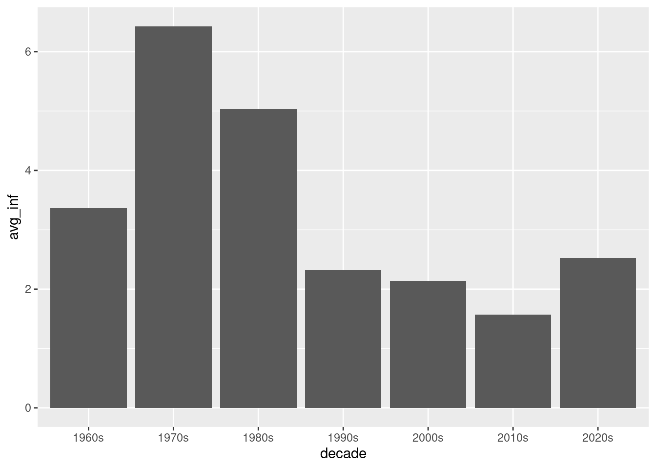
if (!require(pacman)) install.packages("pacman")pacman::p_load(tidyverse, janitor, expss)# setwd("~/yourdirectory-of-choice")rm(list =ls())# read in raw data# PCEPI <- read.csv("PCEPI.csv")PCEPI <-read.csv("https://raw.githubusercontent.com/hubchev/courses/main/dta/PCEPI.csv")# clean datapce_cl <- PCEPI |>mutate(pce = PCEPI_NBD20190101/100) |>mutate(year =str_sub(DATE, 1, 4)) |>mutate(year =as.integer(year)) |>select(pce, year) # make a plotpce_cl |>ggplot( aes(x=year, y=pce))+geom_line() +geom_point()# make a barplotpce_cl |>ggplot( aes(x=year, y=pce))+geom_bar(stat="identity")# make a plot for all years from 2000 onwardspce_cl |>filter(year >2000 ) |>ggplot( aes(x=year, y=pce)) +geom_bar(stat="identity")# make a plot for all years except the 90spce_cl |>filter(year >2000| year <1990) |>ggplot( aes(x=year, y=pce)) +geom_bar(stat="identity")# calculate yearly inflationpce_cl <- pce_cl |>mutate(inflation_rate = (pce/lag(pce)-1)*100 )# plot the inflation ratepce_cl |>ggplot( aes(x=year, y=inflation_rate))+geom_bar(stat="identity")# what is the avergage inflation ratepce_cl |>summarize(avg_mpg =mean(inflation_rate, na.rm =TRUE))# make a variable that indicates the decades 1 for 60s, 2 for 70s, etc.pce_cl <- pce_cl |>mutate(decade =case_when( year <1970~"1960s", (year >1969& year <1980) ~"1970s", (year >1979& year <1990) ~"1980s", (year >1989& year <2000) ~"1990s", (year >1999& year <2010) ~"2000s", (year >2009& year <2020) ~"2010s", (year >2019& year <2030) ~"2020s", )) pce_decade <- pce_cl |>group_by(decade) |>summarize(avg_inf =mean(inflation_rate, na.rm =TRUE)) pce_decadepce_decade |>ggplot( aes(x=decade, y=avg_inf))+geom_bar(stat="identity")
Output of the R script
if (!require(pacman)) install.packages("pacman")pacman::p_load(tidyverse, janitor, expss)# setwd("~/yourdirectory-of-choice")rm(list =ls())# read in raw data# PCEPI <- read.csv("PCEPI.csv")PCEPI <-read.csv("https://raw.githubusercontent.com/hubchev/courses/main/dta/PCEPI.csv")# clean datapce_cl <- PCEPI |>mutate(pce = PCEPI_NBD20190101/100) |>mutate(year =str_sub(DATE, 1, 4)) |>mutate(year =as.integer(year)) |>select(pce, year) # make a plotpce_cl |>ggplot( aes(x=year, y=pce))+geom_line() +geom_point()
# make a barplotpce_cl |>ggplot( aes(x=year, y=pce))+geom_bar(stat="identity")
# make a plot for all years from 2000 onwardspce_cl |>filter(year >2000 ) |>ggplot( aes(x=year, y=pce)) +geom_bar(stat="identity")
# make a plot for all years except the 90spce_cl |>filter(year >2000| year <1990) |>ggplot( aes(x=year, y=pce)) +geom_bar(stat="identity")
Warning: Removed 1 row containing missing values or values outside the scale range
(`geom_bar()`).
# what is the avergage inflation ratepce_cl |>summarize(avg_mpg =mean(inflation_rate, na.rm =TRUE))
   avg_mpg
1 3.454529
# make a variable that indicates the decades 1 for 60s, 2 for 70s, etc.pce_cl <- pce_cl |>mutate(decade =case_when( year <1970~"1960s", (year >1969& year <1980) ~"1970s", (year >1979& year <1990) ~"1980s", (year >1989& year <2000) ~"1990s", (year >1999& year <2010) ~"2000s", (year >2009& year <2020) ~"2010s", (year >2019& year <2030) ~"2020s", )) pce_decade <- pce_cl |>group_by(decade) |>summarize(avg_inf =mean(inflation_rate, na.rm =TRUE)) pce_decade
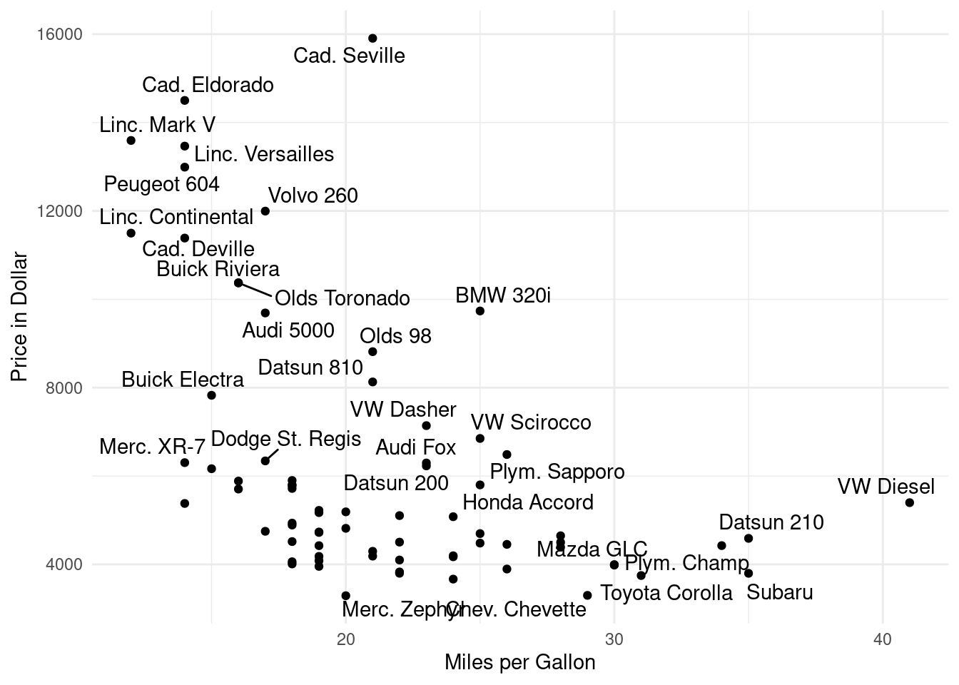
Create a scatter plot illustrating the relationship between the price and weight of a car. Provide a meaningful title for the graph and try to make it clear which car each observation corresponds to.
Save this graph in the formats of .png and .pdf.
Create a variable lp100km that indicates the fuel consumption of an average car in liters per 100 kilometers. (Note: One gallon is approximately equal to 3.8 liters, and one mile is about 1.6 kilometers.)
Create a dummy variable larger6000 that is equal to 1 if the price of a car is above $6000.
Now, search for the “most unreasonable poser car” that costs no more than $6000. A poser car is defined as one that is expensive, has a large turning radius, consumes a lot of fuel, and is often defective (rep78 is low). For this purpose, create a metric indicator for each corresponding variable that indicates a value of 1 for the car that is the most unreasonable in that variable and 0 for the most reasonable car. All other cars should fall between 0 and 1.
Solution
The script uses the following functions: aes, arrange, desc, dir.create, dir.exists, filter, geom_point, geom_text_repel, ggplot, head, ifelse, max, min, min_max_norm, mutate, na.omit, read_dta, select, tail, theme_minimal, xlab, ylab.
R script
# Load the required librariesif (!require(pacman)) install.packages("pacman")pacman::p_load(tidyverse, haven, ggrepel)# setwd("~/Dropbox/hsf/23-ws/R_begin")rm(list =ls())# Read the Stata datasetauto <-read_dta("http://www.stata-press.com/data/r8/auto.dta")# Create a scatter plot of price vs. weightscatter_plot <-ggplot(auto, aes(x = mpg, y = price, label = make)) +geom_point() +geom_text_repel() +xlab("Miles per Gallon") +ylab("Price in Dollar") +theme_minimal()scatter_plot# Create "fig" directory if it doesn't already existif (!dir.exists("fig")) {dir.create("fig")}# Save the scatter plot in different formats# ggsave("fig/scatter_plot.png", plot = scatter_plot, device = "png")# ggsave("fig/scatter_plot.pdf", plot = scatter_plot, device = "pdf")# Create 'lp100km' variable for fuel consumptionn_auto <- auto |>mutate(lp100km = (1/ (mpg *1.6/3.8)) *100)# Create 'larger6000' dummy variablen_auto <- n_auto |>mutate(larger6000 =ifelse(price >6000, 1, 0))# Normalize variables## Do it slowlyn_auto <- n_auto |>mutate(sprice = (price -min(auto$price)) / (max(auto$price) -min(auto$price)))n_auto <- n_auto |>filter(larger6000 ==0)## Do it with a self-written functionmin_max_norm <-function(x) { (x -min(x, na.rm =TRUE)) / (max(x, na.rm =TRUE) -min(x, na.rm =TRUE))}n_auto <- n_auto |>mutate(smpg =min_max_norm(mpg)) |>mutate(sturn =min_max_norm(turn)) |>mutate(slp100km =min_max_norm(lp100km)) |>mutate(sprice =min_max_norm(price)) |>mutate(srep78 =min_max_norm(rep78))## With a loop:# vars_to_normalize <- c("mpg", "turn", "lp100km", "price", "rep78")## # Loop through the selected variables and apply min_max_norm# for (var in c("mpg", "turn", "lp100km", "price", "rep78")) {# auto <- auto |># mutate(!!paste0("s", var) := min_max_norm(!!sym(var))) |># select(make, starts_with("s"))# }## mpg and rep78 need to be changed because a SMALL value is poser-liken_auto <- n_auto |>mutate(smpg =1- smpg) |>mutate(srep78 =1- srep78)## create the poser (composite) indicatorn_auto <- n_auto |>mutate(poser = (sturn + smpg + sprice + srep78) /4)## filter resultsn_auto |>arrange(desc(poser)) |>select(make, poser) |>head(5)df_poser <- n_auto |>filter(larger6000 ==0) |>arrange(desc(poser)) |>select(make, poser) |>na.omit()# Five top poser carshead(df_poser, 15)# Five top non-poser carstail(df_poser, 5)# unload packagessuppressMessages(pacman::p_unload(tidyverse, haven, ggrepel))
Output of the R script
# Load the required librariesif (!require(pacman)) install.packages("pacman")pacman::p_load(tidyverse, haven, ggrepel)# setwd("~/Dropbox/hsf/23-ws/R_begin")rm(list =ls())# Read the Stata datasetauto <-read_dta("http://www.stata-press.com/data/r8/auto.dta")# Create a scatter plot of price vs. weightscatter_plot <-ggplot(auto, aes(x = mpg, y = price, label = make)) +geom_point() +geom_text_repel() +xlab("Miles per Gallon") +ylab("Price in Dollar") +theme_minimal()scatter_plot
Warning: ggrepel: 43 unlabeled data points (too many overlaps). Consider
increasing max.overlaps
# Create "fig" directory if it doesn't already existif (!dir.exists("fig")) {dir.create("fig")}# Save the scatter plot in different formats# ggsave("fig/scatter_plot.png", plot = scatter_plot, device = "png")# ggsave("fig/scatter_plot.pdf", plot = scatter_plot, device = "pdf")# Create 'lp100km' variable for fuel consumptionn_auto <- auto |>mutate(lp100km = (1/ (mpg *1.6/3.8)) *100)# Create 'larger6000' dummy variablen_auto <- n_auto |>mutate(larger6000 =ifelse(price >6000, 1, 0))# Normalize variables## Do it slowlyn_auto <- n_auto |>mutate(sprice = (price -min(auto$price)) / (max(auto$price) -min(auto$price)))n_auto <- n_auto |>filter(larger6000 ==0)## Do it with a self-written functionmin_max_norm <-function(x) { (x -min(x, na.rm =TRUE)) / (max(x, na.rm =TRUE) -min(x, na.rm =TRUE))}n_auto <- n_auto |>mutate(smpg =min_max_norm(mpg)) |>mutate(sturn =min_max_norm(turn)) |>mutate(slp100km =min_max_norm(lp100km)) |>mutate(sprice =min_max_norm(price)) |>mutate(srep78 =min_max_norm(rep78))## With a loop:# vars_to_normalize <- c("mpg", "turn", "lp100km", "price", "rep78")## # Loop through the selected variables and apply min_max_norm# for (var in c("mpg", "turn", "lp100km", "price", "rep78")) {# auto <- auto |># mutate(!!paste0("s", var) := min_max_norm(!!sym(var))) |># select(make, starts_with("s"))# }## mpg and rep78 need to be changed because a SMALL value is poser-liken_auto <- n_auto |>mutate(smpg =1- smpg) |>mutate(srep78 =1- srep78)## create the poser (composite) indicatorn_auto <- n_auto |>mutate(poser = (sturn + smpg + sprice + srep78) /4)## filter resultsn_auto |>arrange(desc(poser)) |>select(make, poser) |>head(5)
# A tibble: 5 × 2
  make             poser
  <chr>            <dbl>
1 Dodge Magnum     0.888
2 Pont. Firebird   0.782
3 Merc. Cougar     0.763
4 Buick LeSabre    0.754
5 Pont. Grand Prix 0.720
df_poser <- n_auto |>filter(larger6000 ==0) |>arrange(desc(poser)) |>select(make, poser) |>na.omit()# Five top poser carshead(df_poser, 15)
Load the packages datasauRus and tidyverse. If necessary, install these packages.
The packagedatasauRus comes with a dataset in two different formats: datasaurus_dozen and datasaurus_dozen_wide. Store them as ds and ds_wide.
Open and read the R vignette of the datasauRus package. Also open the R documentation of the dataset datasaurus_dozen.
Explore the dataset: What are the dimensions of this dataset? Look at the descriptive statistics.
How many unique values does the variable dataset of the tibble ds have? Hint: The function unique() return the unique values of a variable and the function length() returns the length of a vector, such as the unique elements.
Compute the mean values of the x and y variables for each entry in dataset. Hint: Use the group_by() function to group the data by the appropriate column and then the summarise() function to calculate the mean.
Compute the standard deviation, the correlation, and the median in the same way. Round the numbers.
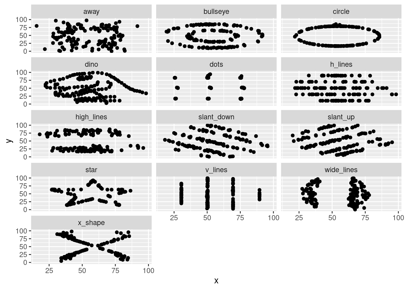
What can you conclude?
Plot all datasets of ds. Hide the legend. Hint: Use the facet_wrap() and the theme() function.
Create a loop that generates separate scatter plots for each unique datatset of the tibble ds. Export each graph as a png file.
# setwd("/home/sthu/Dropbox/hsf/23-ws/ds_mim/")rm(list =ls())# Load the packages datasauRus and tidyverse. If necessary, install these packages.# load packagesif (!require(pacman)) install.packages("pacman")pacman::p_load(datasauRus, tidyverse)# The packagedatasauRus comes with a dataset in two different formats:# datasaurus_dozen and datasaurus_dozen_wide. Store them as ds and ds_wide.ds <- datasaurus_dozends_wide <- datasaurus_dozen_wide# Open and read the R vignette of the datasauRus package.# Also open the R documentation of the dataset datasaurus_dozen.??datasaurus# Explore the dataset: What are the dimensions of this dataset? Look at the descriptive statistics.dsdim(ds)head(ds)glimpse(ds)view(ds)summary(ds)# How many unique values does the variable dataset of the tibble ds have?# Hint: The function unique() return the unique values of a variable and the# function length() returns the length of a vector, such as the unique elements.unique(ds$dataset)unique(ds$dataset) |>length()# Compute the mean values of the x and y variables for each entry in dataset.# Hint: Use the group_by() function to group the data by the appropriate column and# then the summarise() function to calculate the mean.ds |>group_by(dataset) |>summarise(mean_x =mean(x),mean_y =mean(y) )# Compute the standard deviation, the correlation, and the median in the same way. Round the numbers.ds |>group_by(dataset) |>summarise(mean_x =round(mean(x), 2),mean_y =round(mean(y), 2),sd_x =round(sd(x), 2),sd_y =round(sd(y), 2),med_x =round(median(x), 2),med_y =round(median(y), 2),cor =round(cor(x, y), digits =4) )# What can you conclude?# --> The standard deviation, the mean, and the correlation are basically the# same for all datasets. The median is different.# Plot all datasets of ds. Hide the legend. Hint: Use the facet_wrap() and the theme() function.ggplot(ds, aes(x = x, y = y)) +geom_point() +facet_wrap(~dataset, ncol =3) +theme(legend.position ="none")# Create a loop that generates separate scatter plots for each unique datatset of the tibble ds.# Export each graph as a png file.# Assuming uni_ds is a vector of unique values for the 'dataset' variableuni_ds <-unique(ds$dataset)# Create the 'pic' folder if it doesn't existif (!dir.exists("fig")) {dir.create("fig")}for (uni_v in uni_ds) {# Select data for the current value subset_ds <- ds |>filter(dataset == uni_v) |>select(x, y)# Make plot graph <-ggplot(subset_ds, aes(x = x, y = y)) +geom_point() +labs(title =paste("Dataset:", uni_v),x ="X",y ="Y" ) +theme_bw()# Save the plot as a PNG file filename <-paste0("fig/", "plot_ds_", uni_v, ".png")ggsave(filename, plot = graph)}# unload packagessuppressMessages(pacman::p_unload(datasauRus, tidyverse))
Output of the R script
# setwd("/home/sthu/Dropbox/hsf/23-ws/ds_mim/")rm(list =ls())# Load the packages datasauRus and tidyverse. If necessary, install these packages.# load packagesif (!require(pacman)) install.packages("pacman")pacman::p_load(datasauRus, tidyverse)# The packagedatasauRus comes with a dataset in two different formats:# datasaurus_dozen and datasaurus_dozen_wide. Store them as ds and ds_wide.ds <- datasaurus_dozends_wide <- datasaurus_dozen_wide# Open and read the R vignette of the datasauRus package.# Also open the R documentation of the dataset datasaurus_dozen.??datasaurus# Explore the dataset: What are the dimensions of this dataset? Look at the descriptive statistics.ds
   dataset                x               y
 Length:1846        Min.   :15.56   Min.   : 0.01512
 Class :character   1st Qu.:41.07   1st Qu.:22.56107
 Mode  :character   Median :52.59   Median :47.59445
                    Mean   :54.27   Mean   :47.83510
                    3rd Qu.:67.28   3rd Qu.:71.81078
                    Max.   :98.29   Max.   :99.69468
# How many unique values does the variable dataset of the tibble ds have?# Hint: The function unique() return the unique values of a variable and the# function length() returns the length of a vector, such as the unique elements.unique(ds$dataset)
# Compute the mean values of the x and y variables for each entry in dataset.# Hint: Use the group_by() function to group the data by the appropriate column and# then the summarise() function to calculate the mean.ds |>group_by(dataset) |>summarise(mean_x =mean(x),mean_y =mean(y) )
# Compute the standard deviation, the correlation, and the median in the same way. Round the numbers.ds |>group_by(dataset) |>summarise(mean_x =round(mean(x), 2),mean_y =round(mean(y), 2),sd_x =round(sd(x), 2),sd_y =round(sd(y), 2),med_x =round(median(x), 2),med_y =round(median(y), 2),cor =round(cor(x, y), digits =4) )
# What can you conclude?# --> The standard deviation, the mean, and the correlation are basically the# same for all datasets. The median is different.# Plot all datasets of ds. Hide the legend. Hint: Use the facet_wrap() and the theme() function.ggplot(ds, aes(x = x, y = y)) +geom_point() +facet_wrap(~dataset, ncol =3) +theme(legend.position ="none")
# Create a loop that generates separate scatter plots for each unique datatset of the tibble ds.# Export each graph as a png file.# Assuming uni_ds is a vector of unique values for the 'dataset' variableuni_ds <-unique(ds$dataset)# Create the 'pic' folder if it doesn't existif (!dir.exists("fig")) {dir.create("fig")}for (uni_v in uni_ds) {# Select data for the current value subset_ds <- ds |>filter(dataset == uni_v) |>select(x, y)# Make plot graph <-ggplot(subset_ds, aes(x = x, y = y)) +geom_point() +labs(title =paste("Dataset:", uni_v),x ="X",y ="Y" ) +theme_bw()# Save the plot as a PNG file filename <-paste0("fig/", "plot_ds_", uni_v, ".png")ggsave(filename, plot = graph)}
Saving 7 x 5 in image
Saving 7 x 5 in image
Saving 7 x 5 in image
Saving 7 x 5 in image
Saving 7 x 5 in image
Saving 7 x 5 in image
Saving 7 x 5 in image
Saving 7 x 5 in image
Saving 7 x 5 in image
Saving 7 x 5 in image
Saving 7 x 5 in image
Saving 7 x 5 in image
Saving 7 x 5 in image
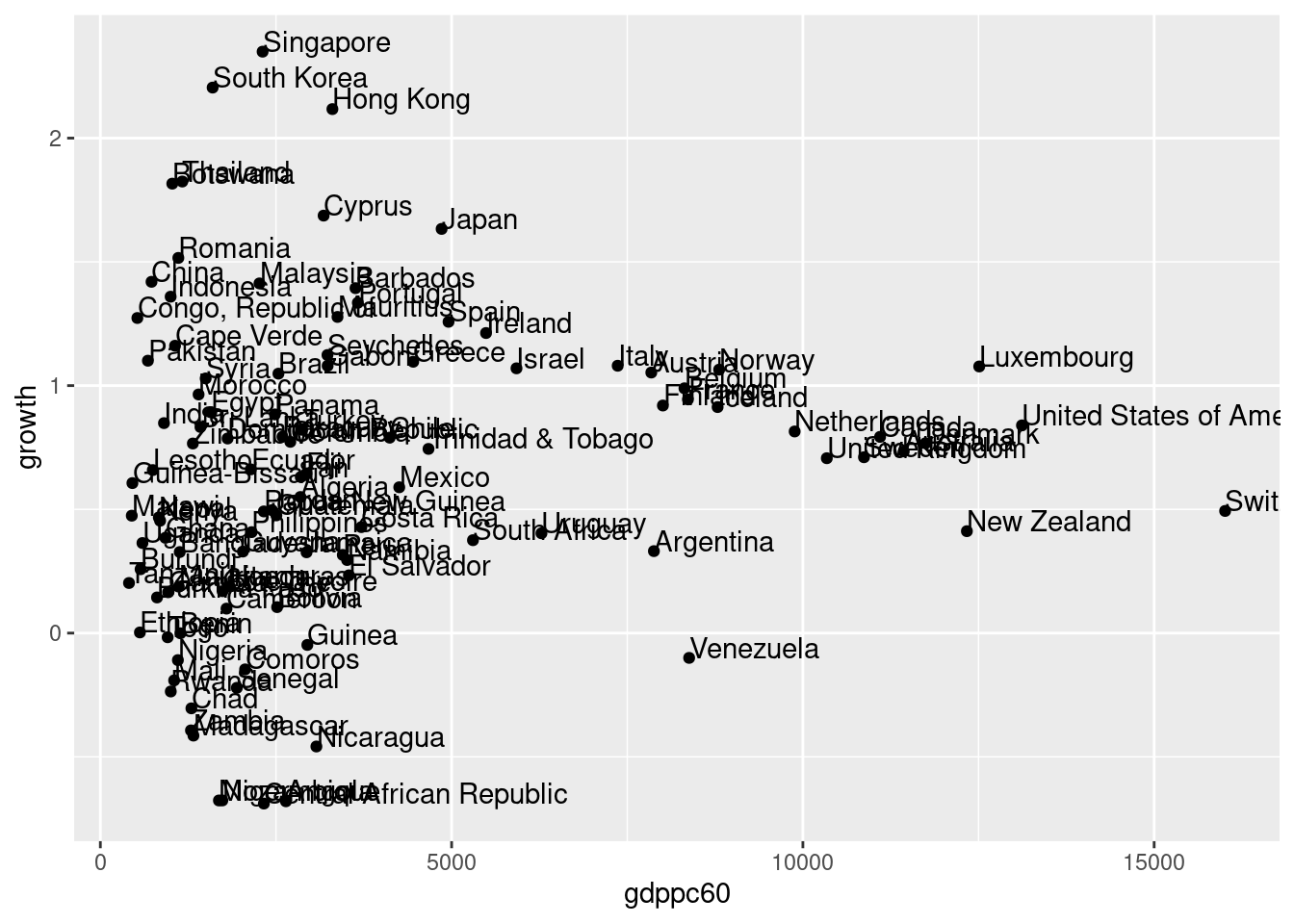
The dataset convergence.dta, see https://github.com/hubchev/courses/blob/main/dta/convergence.dta, contains the per capita GDP of 1960 (gdppc60) and the average growth rate of GDP per capita between 1960 and 1995 (growth) for different countries (country), as well as 3 dummy variables indicating the belonging of a country to the region Asia (asia), Western Europe (weurope) or Africa (africa).
Some countries are not assigned to a certain country group. Name the countries which are assign to be part of Western Europe, Africa or Asia. If you find countries that are members of the EU, assign them a ‘1’ in the variable weurope.
Create a table that shows the average GDP per capita for all available points in time. Group by Western European, Asian, African, and the remaining countries.
Create the growth rate of GDP per capita from 1960 to 1995 and call it gdpgrowth. (Note: The log value X minus the log value X of the previous period is approximately equal to the growth rate).
Calculate the unconditional convergence of all countries by constructing a graph in which a scatterplot shows the GDP per capita growth rate between 1960 and 1995 (gdpgrowth) on the y-axis and the 1960 GDP per capita (gdppc60) on the x-axis. Add to the same graph the estimated linear relationship. You do not need to label the graph further, just two things: title the graph world and label the individual observations with the country names.
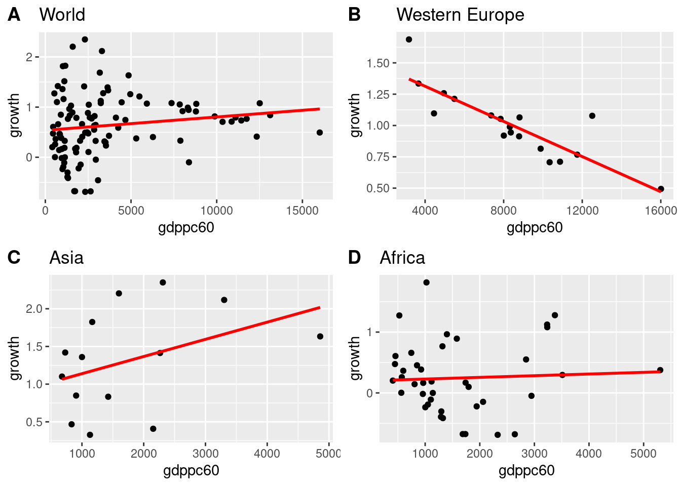
Create three graphs describing the same relationship for the sample of Western European, African and Asian countries. Title the graph accordingly with weurope, africa and asia.
Combine the four graphs into one image. Discuss how an upward or downward sloping regression line can be interpreted.
Estimate the relationships illustrated in the 4 graphs using the least squares method. Present the 4 estimation results in a table, indicating the significance level with stars. In addition, the Akaike information criterion, and the number of observations should be displayed in the table. Interpret the four estimation results regarding their significance.
Put the data set into the so-called long format and calculate the GDP per capita growth rates for the available time points in the countries.
# In the following, I do the same with a loop# c_europe <- c("Austria","Greece","Cyprus")# sum(data$weurope) # check changes# for (i in c_europe){# print(i)# data$weurope[data$country == i] <- 1# }# sum(data$weurope) # check changes# data$weurope[data$country == "Austria"] # check changes# create a category for the remaining countries# use ifelse -- ifelse(condition, result if TRUE, result if FALSE)data$rest <-ifelse(data$africa ==0& data$asia ==0& data$weurope ==0, 1, 0)data$rest <-set_label(data$rest, label ="=1 if not in Africa, W.Europe, or Asia")# create table with means across country groupstable_gdp <- data |>group_by(africa, asia, weurope) |>summarise_at(vars(gdppc60:gdppc95), list(name = mean))data |>group_by(africa, asia, weurope) |>select(gdppc60:gdppc95) |>summarise_all(mean)
p1 <-ggplot(data, aes(x = gdppc60, y = growth, label = country)) +geom_point() +stat_smooth(formula = y ~ x, method ="lm", se =FALSE, colour ="red", linetype =1) +# geom_text(hjust=0, vjust=0) +ggtitle("World")p2 <- data |>filter(weurope ==1) |>ggplot(aes(x = gdppc60, y = growth, label = country)) +geom_point() +stat_smooth(formula = y ~ x, method ="lm", se =FALSE, colour ="red", linetype =1) +# geom_text(hjust=0, vjust=0) +ggtitle("Western Europe")p3 <- data |>filter(asia ==1) |>ggplot(aes(x = gdppc60, y = growth, label = country)) +geom_point() +stat_smooth(formula = y ~ x, method ="lm", se =FALSE, colour ="red", linetype =1) +# geom_text(hjust=0, vjust=0) +ggtitle("Asia")p4 <- data |>filter(africa ==1) |>ggplot(aes(x = gdppc60, y = growth, label = country)) +geom_point() +stat_smooth(formula = y ~ x, method ="lm", se =FALSE, colour ="red", linetype =1) +# geom_text( hjust=0, vjust=0) +ggtitle("Africa")ggarrange(p1, p2, p3, p4,labels =c("A", "B", "C", "D"),ncol =2, nrow =2)
Warning: The following aesthetics were dropped during statistical transformation: label.
ℹ This can happen when ggplot fails to infer the correct grouping structure in
the data.
ℹ Did you forget to specify a `group` aesthetic or to convert a numerical
variable into a factor?
The following aesthetics were dropped during statistical transformation: label.
ℹ This can happen when ggplot fails to infer the correct grouping structure in
the data.
ℹ Did you forget to specify a `group` aesthetic or to convert a numerical
variable into a factor?
The following aesthetics were dropped during statistical transformation: label.
ℹ This can happen when ggplot fails to infer the correct grouping structure in
the data.
ℹ Did you forget to specify a `group` aesthetic or to convert a numerical
variable into a factor?
The following aesthetics were dropped during statistical transformation: label.
ℹ This can happen when ggplot fails to infer the correct grouping structure in
the data.
ℹ Did you forget to specify a `group` aesthetic or to convert a numerical
variable into a factor?
# Regression analysism1 <-lm(growth ~ gdppc60, data = data)m2 <-lm(growth ~ gdppc60, data =subset(data, weurope ==1))m3 <-lm(growth ~ gdppc60, data =subset(data, asia ==1))m4 <-lm(growth ~ gdppc60, data =subset(data, africa ==1))tab_model(m1, m2, m3, m4,p.style ="stars",p.threshold =c(0.2, 0.1, 0.05),show.ci =FALSE,show.se =FALSE,show.aic =TRUE,dv.labels =c("World", "W.Europe", "Asia", "Africa"))
Please answer all (!) questions in an R script. Normal text should be written as comments, using the ‘#’ to comment out text. Make sure the script runs without errors before submitting it. Each task (starting with 1) is worth five points. You have a total of 120 minutes of editing time. Please do not forget to number your answers.
When you are done with your work, save the R script, export the script to pdf format and upload the pdf file.
Suppose you aim to empirically examine unemployment and GDP for Germany and France. The data set that we use in the following is ‘forest.Rdata’.
Write down your name, matriculation number, and date.
Set your working directory.
Clear your global environment.
Install and load the following packages: ‘tidyverse’, ‘sjPlot’, and ‘ggpubr’
Download and load the data, respectively, with the following code:
If that is not working, you can also download the data from ILIAS, save it in your working directory and load it from there with:
# load("forest.Rdata")
Show the first eight observations of the dataset df.
Show the last observation of the dataset df.
Which type of data do we have here (Panel, cross-section,time series, …)? Name the variable(s) that are necessary to identify the observations in the dataset.
Explain what the assignment operator in R is and what it is good for.
Write down the R code to store the number of observations and the number of variables that are in the dataset df. Name the object in which you store these numbers ‘observations_df’.
In the dataset df, rename the variable ‘country.x’ to ‘nation’ and the variable ‘date’ to ‘year’.
Explain what the pipe operator in R is and what it is good for.
For the upcoming analysis you are only interested the following variables that are part of the dataframe df: nation, year, gdp, pop, gdppc, and unemployment. Drop all other variables from the dataframe df.
Create a variable that indicates the GDP per capita (‘gdp’ divided by ‘pop’). Name the variable ‘gdp_pc’. (Hint: If you fail here, use the variable ‘gdppc’ which is already in the dataset as a replacement for ‘gdp_pc’ in the following tasks.)
For the upcoming analysis you are only interested the following countries that are part of the dataframe df: Germany and France. Drop all other countries from the dataframe df.
Create a table showing the average unemployment rate and GDP per capita for Germany and France in the given years. Use the pipe operator. (Hint: See below for how your results should look like.)
# A tibble: 2 × 3
nation `mean(unemployment)` `mean(gdppc)`
<chr> <dbl> <dbl>
1 France 9.75 34356.
2 Germany 7.22 36739.
Create a table showing the unemployment rate and GDP per capita for Germany and France in the year 2020. Use the pipe operator. (Hint: See below for how your results should look like.)
# A tibble: 2 × 3
nation `mean(unemployment)` `mean(gdppc)`
<chr> <dbl> <dbl>
1 France 8.01 35786.
2 Germany 3.81 41315.
Create a table showing the highest unemployment rate and the highest GDP per capita for Germany and France during the given period. Use the pipe operator. (Hint: See below for how your results should look like.)
# A tibble: 2 × 3
nation `max(unemployment)` `max(gdppc)`
<chr> <dbl> <dbl>
1 France 12.6 38912.
2 Germany 11.2 43329.
Calculate the standard deviation of the unemployment rate and GDP per capita for Germany and France in the given years. (Hint: See below for how your result should look like.)
# A tibble: 2 × 3
nation `sd(gdppc)` `sd(unemployment)`
<chr> <dbl> <dbl>
1 France 2940. 1.58
2 Germany 4015. 2.37
In statistics, the coefficient of variation (COV) is a standardized measure of dispersion. It is defined as the ratio of the standard deviation (\(\sigma\)) to the mean (\(\mu\)): \(COV={\frac {\sigma }{\mu }}\). Write down the R code to calculate the coefficient of variation (COV) for the unemployment rate in Germany and France. (Hint: See below for what your result should should look like.)
Write down the R code to calculate the coefficient of variation (COV) for the GDP per capita in Germany and France. (Hint: See below for what your result should look like.)
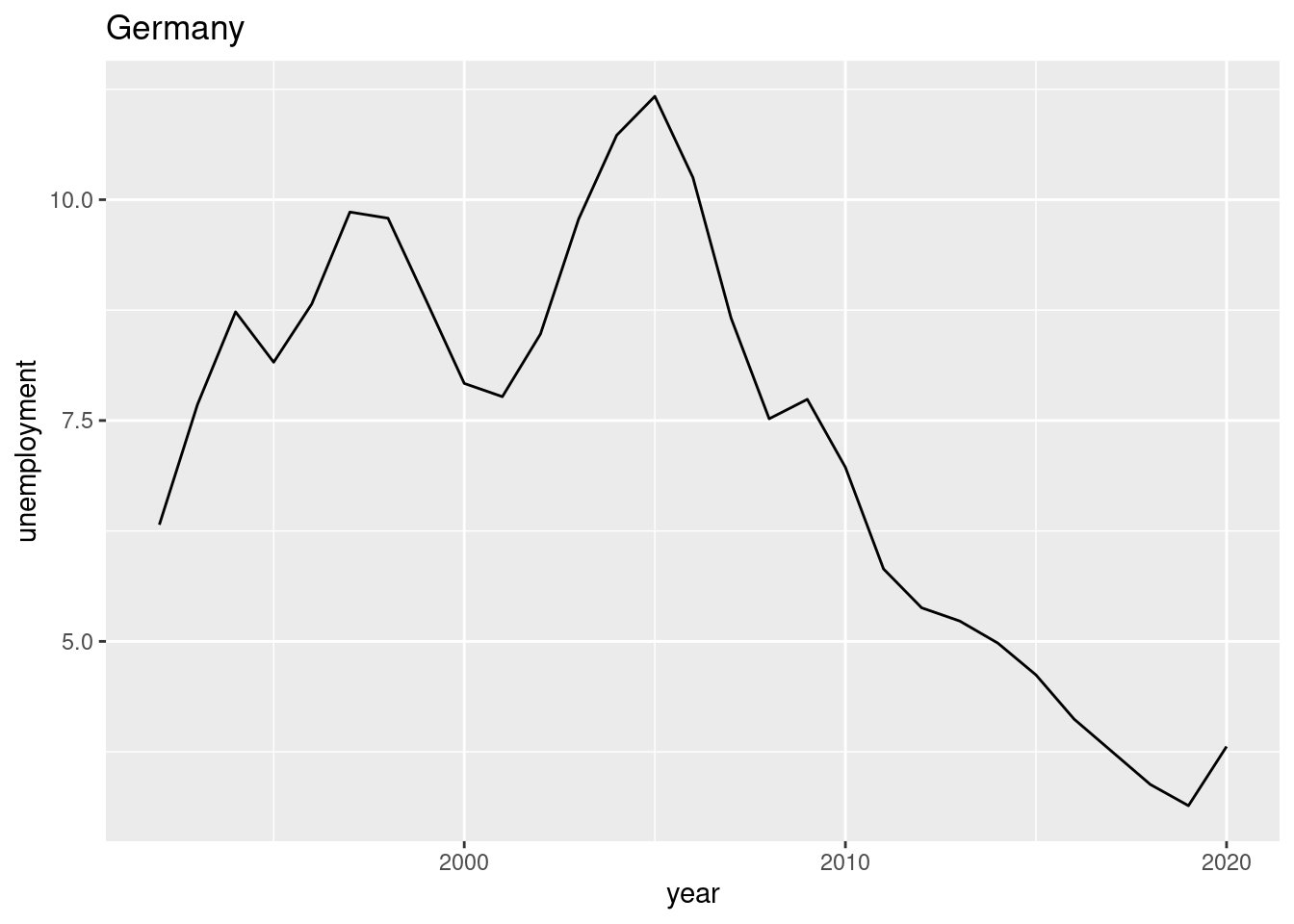
Create a chart (bar chart, line chart, or scatter plot) that shows the unemployment rate of Germany over the available years. Label the chart ‘Germany’ with ‘ggtitle(“Germany”)’. Please note that you may choose any type of graphical representation. (Hint: Below you can see one of many |> of what your result may look like).
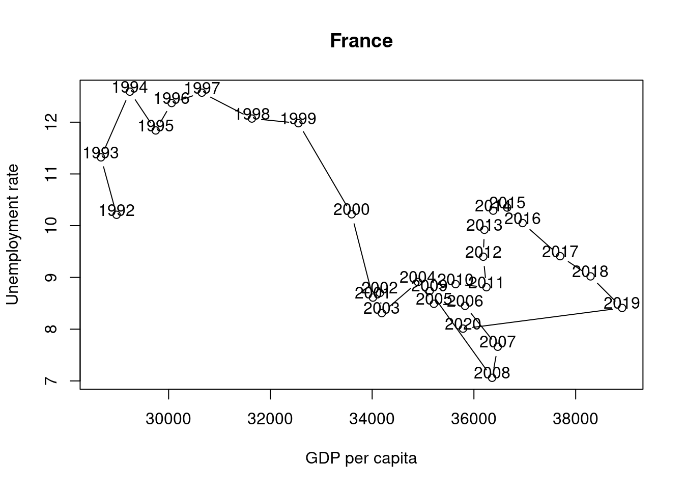
and 23. (This task is worth 10 points) The following chart shows the simultaneous development of the unemployment rate and GDP per capita over time for France.
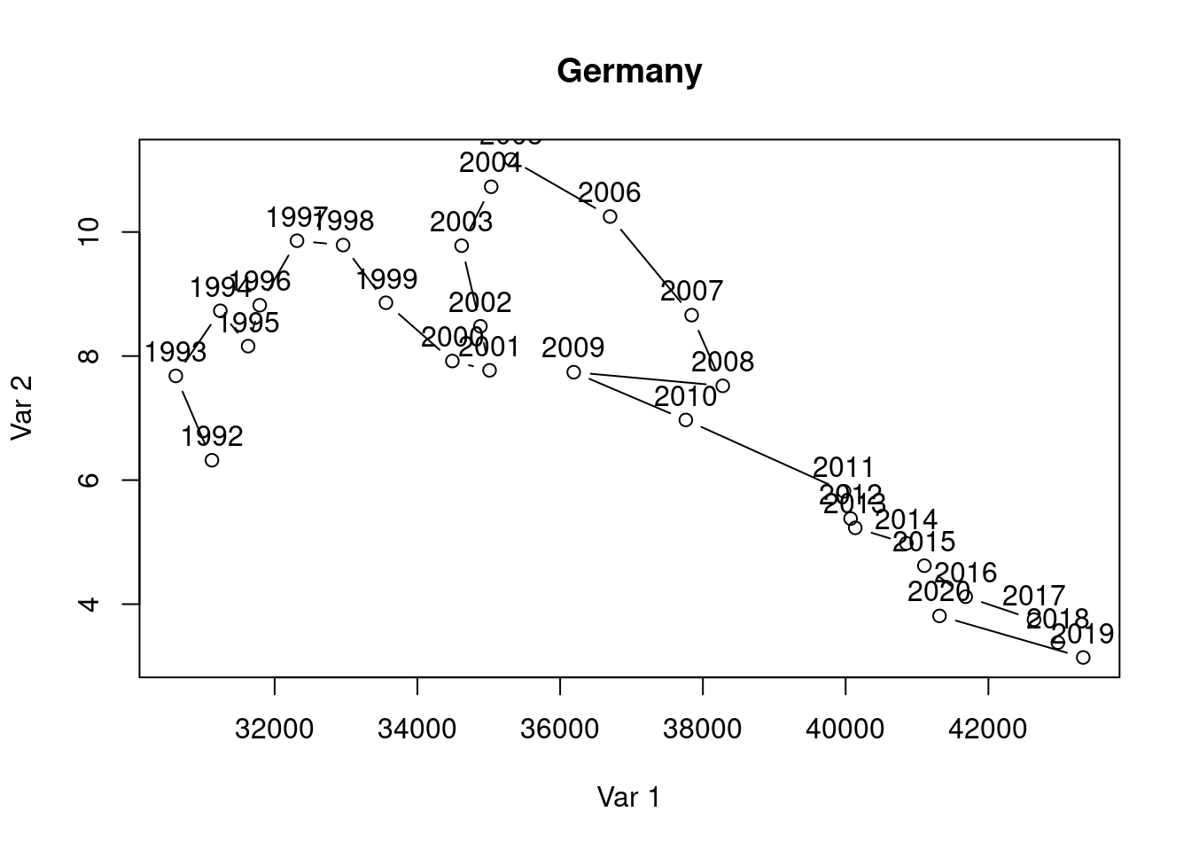
Suppose you want to visualize the simultaneous evolution of the unemployment rate and GDP per capita over time for Germany as well.
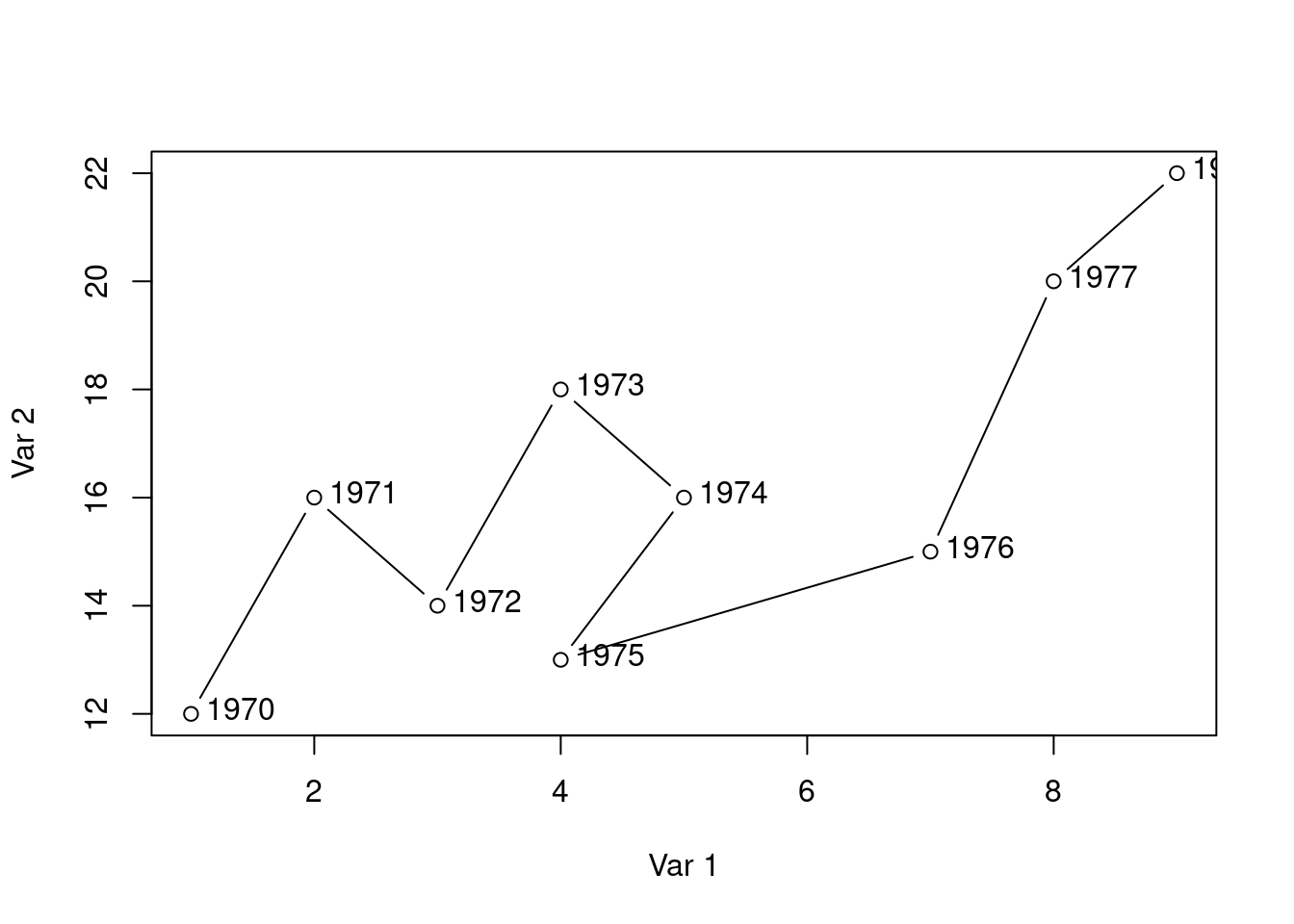
Suppose further that you have found the following lines of code that create the kind of chart you are looking for.
# Datax <-c(1, 2, 3, 4, 5, 4, 7, 8, 9)y <-c(12, 16, 14, 18, 16, 13, 15, 20, 22)labels <-1970:1978# Connected scatter plot with textplot(x, y, type ="b", xlab ="Var 1", ylab ="Var 2")text(x +0.4, y +0.1, labels)
Use these lines of code and customize them to create the co-movement visualization for Germany using the available df data. The result should look something like this:
Interpret the two graphs above, which show the simultaneous evolution of the unemployment rate and GDP per capita over time for Germany and France. What are your expectations regarding the correlation between the unemployment rate and GDP per capita variables? Can you see this expectation in the figures? Discuss.
Solution
The script uses the following functions: aes, c, dim, filter, geom_line, ggplot, ggtitle, group_by, head, load, max, mean, mutate, plot, rename, sd, select, summarise, tail, text, title, url.
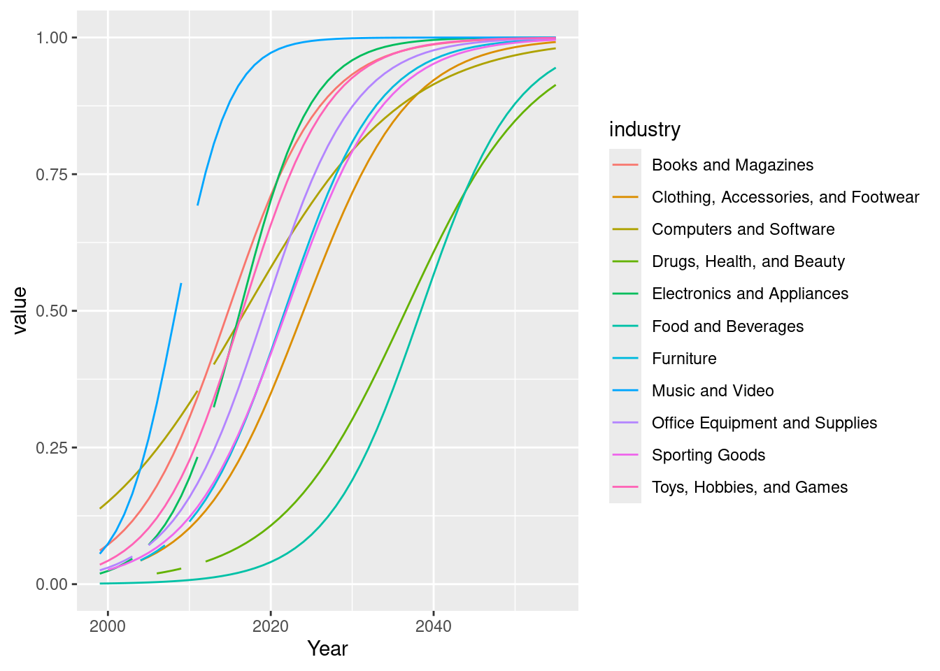
Reproduce Figure 3 of Hortaçsu & Syverson (2015, p. 99) using R. Write a clear report about your work, i.e., document everything with a R script or a R Markdown file.
Hortaçsu, A., & Syverson, C. (2015). The ongoing evolution of US retail: A format tug-of-war. Journal of Economic Perspectives, 29(4), 89–112.
Here are the required steps:
Go to https://www.aeaweb.org/articles?id=10.1257/jep.29.4.89 and download the replication package from the OPENICPSR page. Please note, that you can download the replication package after you have registered for the platform.
Unzip the replication package.
In the file diffusion_curves_figure.xlsx you find the required data. Import them to R.
Reproduce the plot using ggplot().
Solution
The script uses the following functions: aes, download.file, geom_line, ggplot, pivot_longer, read_excel, unzip.
R script
# setwd("~/Dropbox/hsf/courses/Rlang/hortacsu")rm(list =ls())# install and load packagesif (!require(pacman)) install.packages("pacman")pacman::p_load(tidyverse, readxl)# Define the URL of the ZIP filezip_f <-"https://github.com/hubchev/courses/raw/main/dta/113962-V1.zip"# Download the ZIP filedownload.file(zip_f, destfile ="113962-V1.zip")# Unzip the contentsunzip("113962-V1.zip")df_curves <-read_excel("Hortacsu_Syverson_JEP_Retail/diffusion_curves_figure.xlsx",sheet ="Data and Predictions", range ="N3:Y60")df <- df_curves |>pivot_longer(cols ="Music and Video":"Food and Beverages",names_to ="industry",values_to ="value" )# Plotdf |>ggplot(aes(x = Year, y = value, group = industry, color = industry)) +geom_line()# unload packagessuppressMessages(pacman::p_unload(tidyverse, readxl))
Output of the R script
# setwd("~/Dropbox/hsf/courses/Rlang/hortacsu")rm(list =ls())# install and load packagesif (!require(pacman)) install.packages("pacman")pacman::p_load(tidyverse, readxl)# Define the URL of the ZIP filezip_f <-"https://github.com/hubchev/courses/raw/main/dta/113962-V1.zip"# Download the ZIP filedownload.file(zip_f, destfile ="113962-V1.zip")# Unzip the contentsunzip("113962-V1.zip")df_curves <-read_excel("Hortacsu_Syverson_JEP_Retail/diffusion_curves_figure.xlsx",sheet ="Data and Predictions", range ="N3:Y60")df <- df_curves |>pivot_longer(cols ="Music and Video":"Food and Beverages",names_to ="industry",values_to ="value" )# Plotdf |>ggplot(aes(x = Year, y = value, group = industry, color = industry)) +geom_line()
Warning: Removed 18 rows containing missing values or values outside the scale range
(`geom_line()`).
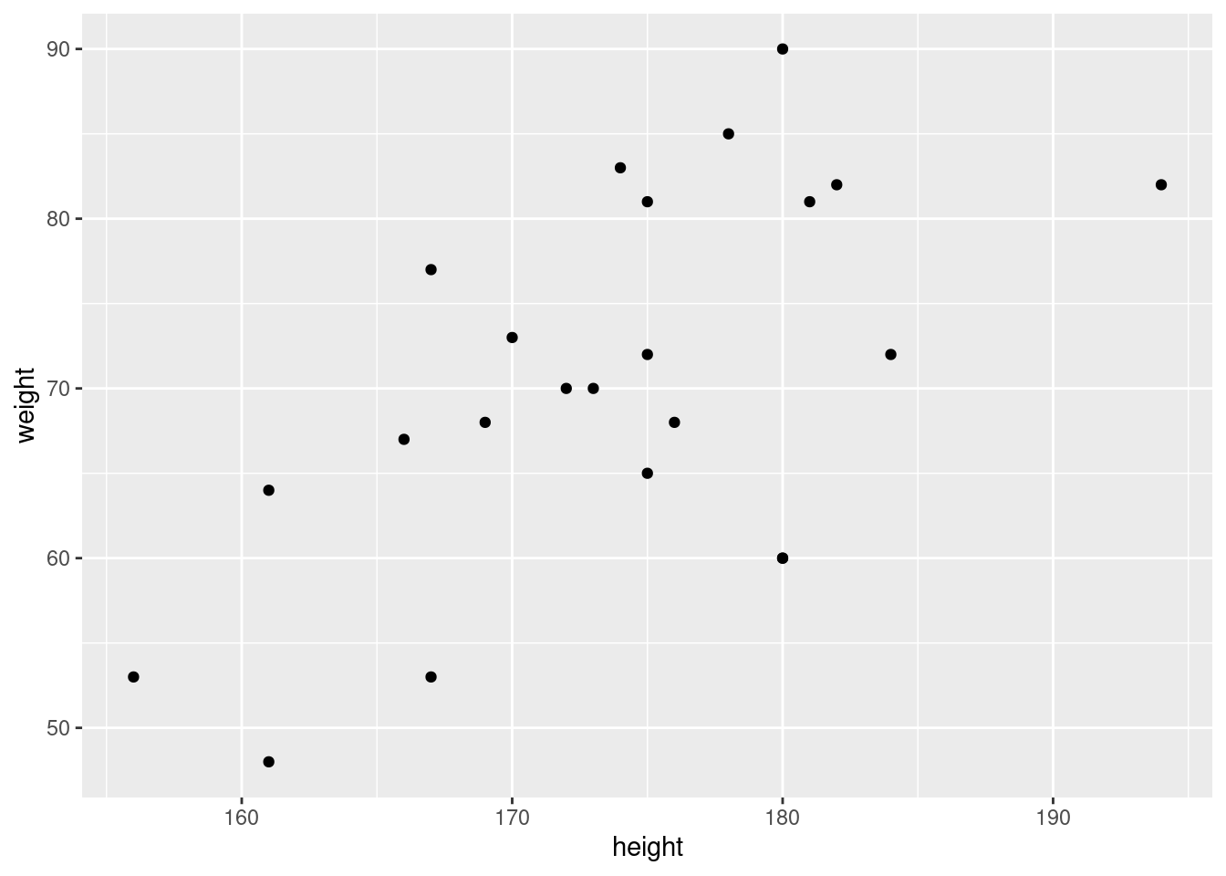
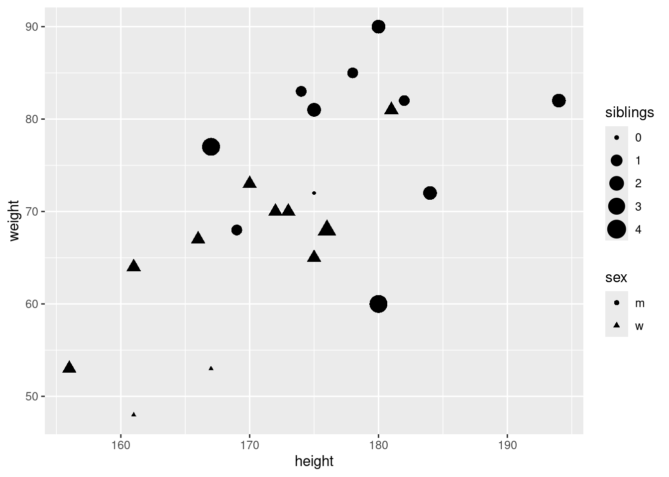
In the statistic course of WS 2020, I asked 23 students about their weight, height, sex, and number of siblings. I wonder how good the height can explain the weight of students. Examine with corelations and a regression analysis the association. Load the data as follows:
library("haven")
Attaching package: 'haven'
The following objects are masked from 'package:expss':
is.labelled, read_spss
id sex weight height
Min. : 1.0 Length:23 Min. :48.00 Min. :156.0
1st Qu.: 6.5 Class :character 1st Qu.:64.50 1st Qu.:168.0
Median :12.0 Mode :character Median :70.00 Median :175.0
Mean :12.0 Mean :70.61 Mean :173.7
3rd Qu.:17.5 3rd Qu.:81.00 3rd Qu.:180.0
Max. :23.0 Max. :90.00 Max. :194.0
siblings row
Min. :0.000 Length:23
1st Qu.:1.000 Class :character
Median :1.000 Mode :character
Mean :1.391
3rd Qu.:2.000
Max. :4.000
## ----pressure, echo=TRUE-------------------------------------------ggplot(classdata, aes(x = height, y = weight)) +geom_point()
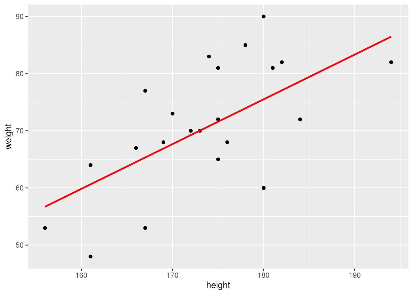
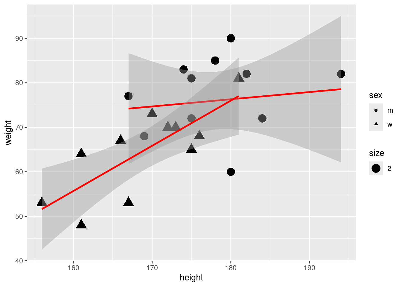
## ---- echo=TRUE----------------------------------------------------ggplot(classdata, aes(x = height, y = weight)) +geom_point() +stat_smooth(formula = y ~ x, method ="lm", se =FALSE, colour ="red", linetype =1)
Write down your name, your matriculation number, and the date.
Set your working directory.
Clear your global environment.
Load the following package: tidyverse
The following table stems from a survey carried out at the Campus of the German Sport University of Cologne at Opening Day (first day of the new semester) between 8:00am and 8:20am. The survey consists of 6 individuals with the following information:
id
sex
age
weight
calories
sport
1
f
21
48
1700
60
2
f
19
55
1800
120
3
f
23
50
2300
180
4
m
18
71
2000
60
5
m
20
77
2800
240
6
m
61
85
2500
30
Data Description:
id: Variable with an anonymized identifier for each participant.
sex: Gender, i.e., the participants replied to be either male (m) or female (f).
age: The age in years of the participants at the time of the survey.
weight: Number of kg the participants pretended to weight.
calories: Estimate of the participants on their average daily consumption of calories.
sport: Estimate of the participants on their average daily time that they spend on doing sports (measured in minutes).
Which type of data do we have here? (Panel data, repeated cross-sectional data, cross-sectional data, time Series data)
Store each of the five variables in a vector and put all five variables into a dataframe with the title df. If you fail here, read in the data using this line of code:
Rows: 6 Columns: 5
── Column specification ────────────────────────────────────────────────────────
Delimiter: ","
chr (1): sex
dbl (4): age, weight, calories, sport
ℹ Use `spec()` to retrieve the full column specification for this data.
ℹ Specify the column types or set `show_col_types = FALSE` to quiet this message.
Show for all numerical variables the summary statistics including the mean, median, minimum, and the maximum.
Show for all numerical variables the summary statistics including the mean and the standard deviation, separated by male and female. Use therefore the pipe operator.
Suppose you want to analyze the general impact of average calories consumption per day on the weight. Discuss if the sample design is appropriate to draw conclusions on the population. What may cause some bias in the data? Discuss possibilities to improve the sampling and the survey, respectively.
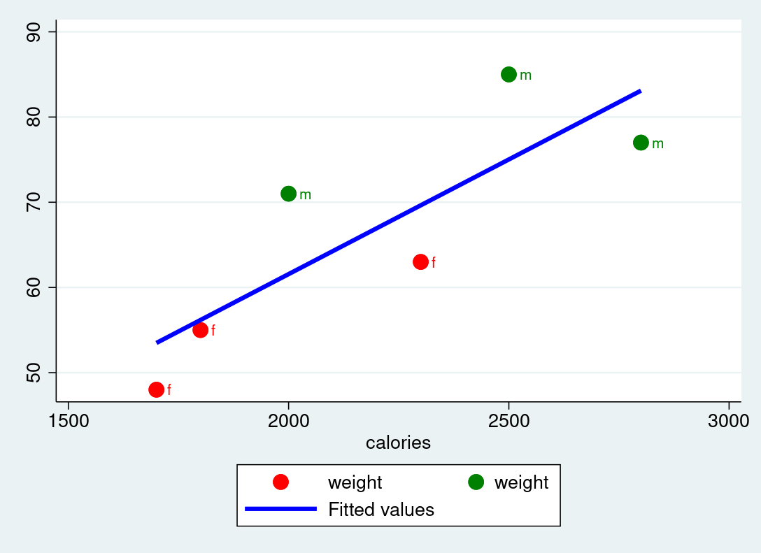
The following plot visualizes the two variables weight and calories. Discuss what can be improved in the graphical visualization.
Weight vs. Calories
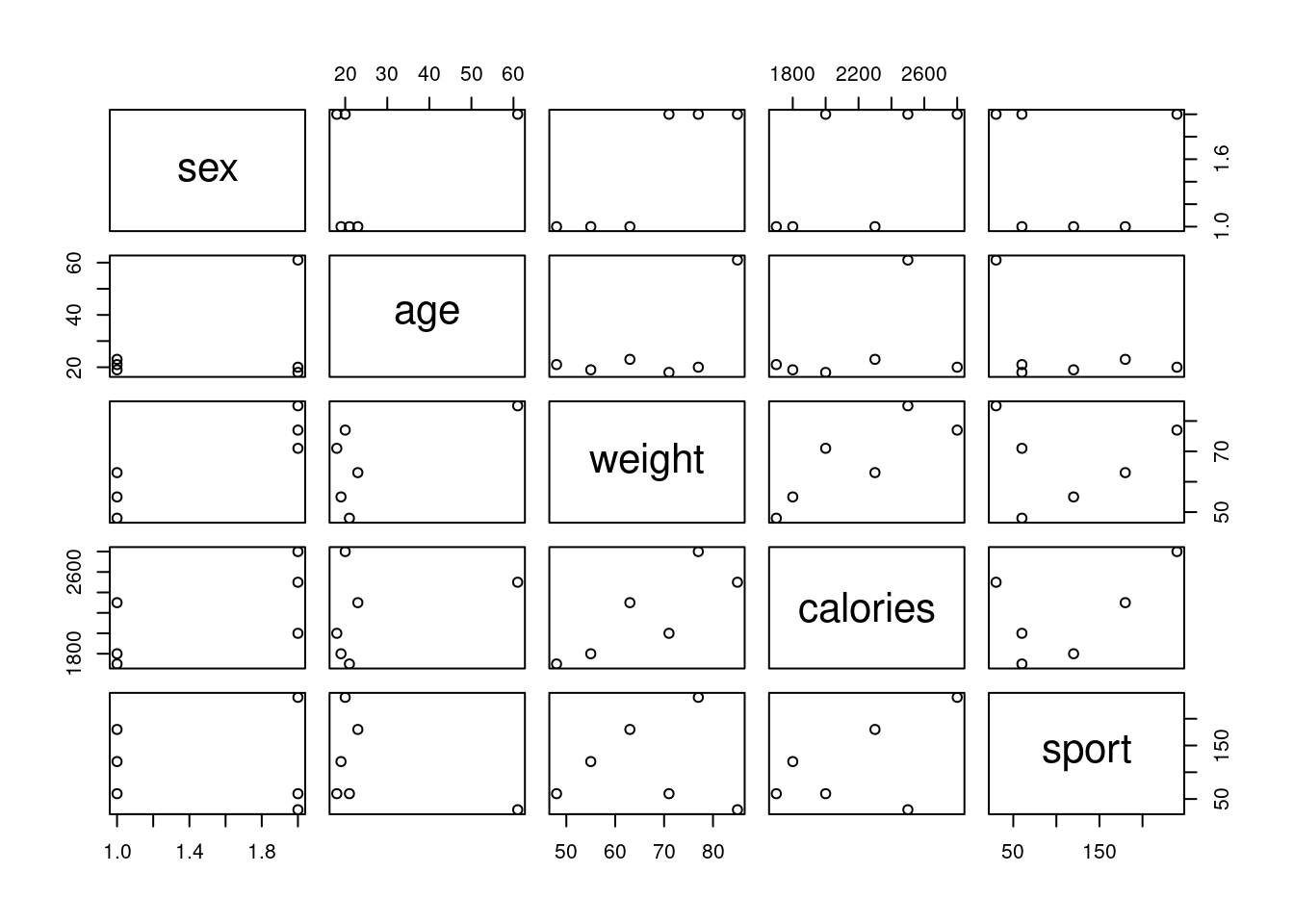
Make a scatterplot matrix containing all numerical variables.
Calculate the Pearson Correlation Coefficient of the two variables
calories and sport
weight and calories
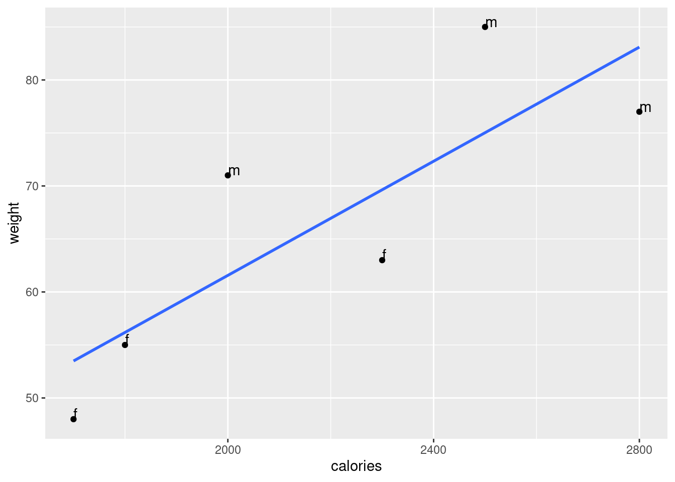
Make a scatterplot with weight in the y-axis and calories on the x-axis. Additionally, the plot should contain a linear fit and the points should be labeled with the sex just like in the figure shown above.
Estimate the following regression specification using the OLS method: [weight_i=_0+_1 calories_i+ _i]
Show a summary of the estimates that look like the following:
Call:
lm(formula = weight ~ calories, data = df)
Residuals:
1 2 3 4 5 6
-5.490 -1.182 -6.640 9.435 -6.099 9.976
Coefficients:
Estimate Std. Error t value Pr(>|t|)
(Intercept) 7.730275 20.197867 0.383 0.7214
calories 0.026917 0.009107 2.956 0.0417 *
---
Signif. codes: 0 '***' 0.001 '**' 0.01 '*' 0.05 '.' 0.1 ' ' 1
Residual standard error: 8.68 on 4 degrees of freedom
Multiple R-squared: 0.6859, Adjusted R-squared: 0.6074
F-statistic: 8.735 on 1 and 4 DF, p-value: 0.04174
Interpret the results. In particular, interpret how many kg the estimated weight increases—on average and ceteris paribus—if calories increase by 100 calories. Additionally, discuss the statistical properties of the estimated coefficient \(\hat{\beta_1}\) and the meaning of the Adjusted R-squared.
OLS estimates can suffer from omitted variable bias. State the two conditions that need to be fulfilled for omitted bias to occur.
Discuss potential confounding variables that may cause omitted variable bias. Given the dataset above how can some of the confounding variables be controlled for?
Solution
The script uses the following functions: aes, c, cor, data.frame, geom_point, geom_text, ggplot, group_by, lm, mean, plot, read_csv, sd, stat_smooth, summarise, summary.
R script
# 1# Stephan Huber, 000, 2020-May-30# 2# setwd("/home/sthu/Dropbox/hsf/22-ss/dsb_bac/work/")# 3rm(list =ls())# 4if (!require(pacman)) install.packages("pacman")pacman::p_load(tidyverse, haven)# 5# cross-section# 6sex <-c("f", "f", "f", "m", "m", "m")age <-c(21, 19, 23, 18, 20, 61)weight <-c(48, 55, 63, 71, 77, 85)calories <-c(1700, 1800, 2300, 2000, 2800, 2500)sport <-c(60, 120, 180, 60, 240, 30)df <-data.frame(sex, age, weight, calories, sport)# write_csv(df, file = "/home/sthu/Dropbox/hsf/exams/21-04/stuff/df.csv")# write_csv(df, file = "/home/sthu/Dropbox/hsf/github/courses/dta/df-calories.csv")df <-read_csv("https://raw.githubusercontent.com/hubchev/courses/main/dta/df-calories.csv")# 7summary(df)# 8df |>group_by(sex) |>summarise(mcal =mean(calories),sdcal =sd(calories),mweight =mean(weight),sdweight =sd(weight) )# 9# discussed in class# 10# Many things can be mentioned here such as the use of colors# (red/blue is not a good choice for color blind people),# the legend makes no sense as red and green both refer to \textit{sport},# the label of `f' and `m' is not explained in the legend,# rotating the labels of the y-axis would increase readability, and# both axes do not start at zero which is hard to see.# Also, it is a common to draw the variable you want to explain# (here: calories) on the y-axis.# 11plot(df)# 12cor(df$calories, df$sport, method =c("pearson"))cor(df$weight, df$calories, method =c("pearson"))# 13ggplot(df, aes(x = calories, y = weight, label = sex)) +geom_point() +geom_text(hjust =0, vjust =0) +stat_smooth(formula = y ~ x, method ="lm", se =FALSE)# 14reg_base <-lm(weight ~ calories, data = df)summary(reg_base)# 15# 1) An increase of 100 calories (taken on average on a daily basis) is associated# - on average and ceteris paribus - with 2.69 more of kg the participants are# pretended to weight.# 2) The estimated coefficient $beta_1$ is statistically significantly different to zero# on a significance level of 5%.# 3) About 60 % of the variation of the weight is explained by the# estimated coefficients of the empirical model.# 16# For omitted variable bias to occur, the omitted variable `Z` must satisfy# two conditions:# 1) The omitted variable is correlated with the included regressor# 2) The omitted variable is a determinant of the dependent variable# 17# discussed in class# unload packagessuppressMessages(pacman::p_unload(tidyverse, haven))
Rows: 6 Columns: 5
── Column specification ────────────────────────────────────────────────────────
Delimiter: ","
chr (1): sex
dbl (4): age, weight, calories, sport
ℹ Use `spec()` to retrieve the full column specification for this data.
ℹ Specify the column types or set `show_col_types = FALSE` to quiet this message.
# 7summary(df)
sex age weight calories sport
Length:6 Min. :18.00 Min. :48.0 Min. :1700 Min. : 30
Class :character 1st Qu.:19.25 1st Qu.:57.0 1st Qu.:1850 1st Qu.: 60
Mode :character Median :20.50 Median :67.0 Median :2150 Median : 90
Mean :27.00 Mean :66.5 Mean :2183 Mean :115
3rd Qu.:22.50 3rd Qu.:75.5 3rd Qu.:2450 3rd Qu.:165
Max. :61.00 Max. :85.0 Max. :2800 Max. :240
# A tibble: 2 × 5
sex mcal sdcal mweight sdweight
<chr> <dbl> <dbl> <dbl> <dbl>
1 f 1933. 321. 55.3 7.51
2 m 2433. 404. 77.7 7.02
# 9# discussed in class# 10# Many things can be mentioned here such as the use of colors# (red/blue is not a good choice for color blind people),# the legend makes no sense as red and green both refer to \textit{sport},# the label of `f' and `m' is not explained in the legend,# rotating the labels of the y-axis would increase readability, and# both axes do not start at zero which is hard to see.# Also, it is a common to draw the variable you want to explain# (here: calories) on the y-axis.# 11plot(df)
# 13ggplot(df, aes(x = calories, y = weight, label = sex)) +geom_point() +geom_text(hjust =0, vjust =0) +stat_smooth(formula = y ~ x, method ="lm", se =FALSE)
Warning: The following aesthetics were dropped during statistical transformation: label.
ℹ This can happen when ggplot fails to infer the correct grouping structure in
the data.
ℹ Did you forget to specify a `group` aesthetic or to convert a numerical
variable into a factor?
# 14reg_base <-lm(weight ~ calories, data = df)summary(reg_base)
Call:
lm(formula = weight ~ calories, data = df)
Residuals:
1 2 3 4 5 6
-5.490 -1.182 -6.640 9.435 -6.099 9.976
Coefficients:
Estimate Std. Error t value Pr(>|t|)
(Intercept) 7.730275 20.197867 0.383 0.7214
calories 0.026917 0.009107 2.956 0.0417 *
---
Signif. codes: 0 '***' 0.001 '**' 0.01 '*' 0.05 '.' 0.1 ' ' 1
Residual standard error: 8.68 on 4 degrees of freedom
Multiple R-squared: 0.6859, Adjusted R-squared: 0.6074
F-statistic: 8.735 on 1 and 4 DF, p-value: 0.04174
# 15# 1) An increase of 100 calories (taken on average on a daily basis) is associated# - on average and ceteris paribus - with 2.69 more of kg the participants are# pretended to weight.# 2) The estimated coefficient $beta_1$ is statistically significantly different to zero# on a significance level of 5%.# 3) About 60 % of the variation of the weight is explained by the# estimated coefficients of the empirical model.# 16# For omitted variable bias to occur, the omitted variable `Z` must satisfy# two conditions:# 1) The omitted variable is correlated with the included regressor# 2) The omitted variable is a determinant of the dependent variable# 17# discussed in class# unload packagessuppressMessages(pacman::p_unload(tidyverse, haven))
9.15 Bundesliga
Open the script that you find here and work on the following tasks:
Set your working directory.
Clear th environment.
Install and load the bundesligR and tidyverse.
Read in the data bundesligR as a tibble.
Replace “Bor. Moenchengladbach” with “Borussia Moenchengladbach.”
Check for the data class.
View the data.
Glimpse on the data.
Show the first and last observations.
Show summary statistics to all variables.
How many teams have played in the league over the years?
Which teams have played Bundesliga so far?
How many teams have played Bundesliga?
How often has each team played in the Bundesliga?
Show summary statistics of variable Season only.
Show summary statistics of all numeric variables (Team is a character).
What is the highest number of points ever received by a team? Show only the name of the club with the highest number of points ever received.
Create a new tibble using liga removing the variable Pts_pre_95 from the data.
Create a new tibble using liga renaming W, D, and L to Win, Draw, and Loss. Additionally rename GF, GA, GD to Goals_shot, Goals_received, Goal_difference.
Create a new tibble using liga without the variable Pts_pre_95 and only observations before the year 1996.
Remove the three tibbles just created from the environment.
Rename all variables of liga to lowercase and store it as dfb.
Show the winner and the runner up after the year 2010. Additionally show the points received.
Create a variable that counts how often a team was ranked first.
How often has each team played in the Bundesliga?
Make a ranking that shows which team has played the Bundesliga most often.
Add a variable to dfb that contains the number of appearances of a team in the league.
Create a number that indicates how often a team has played Bundesliga in a given year.
Make a ranking with the number of titles of all teams that ever won the league.
Create a numeric identifying variable for each team.
When a team is in the league, what is the probability that it wins the league?
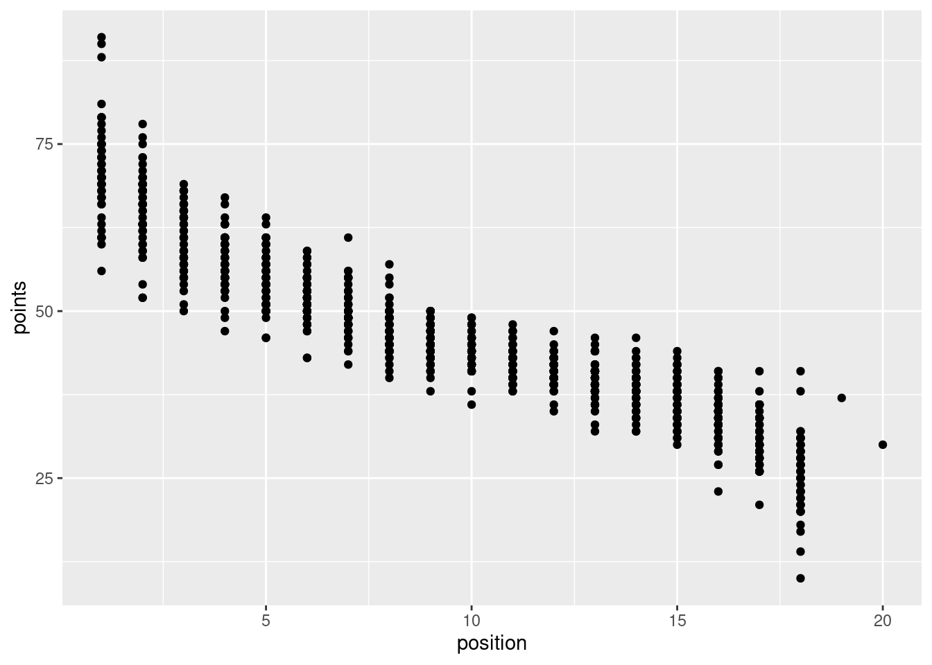
Make a scatterplot with points on the y-axis and position on the x-axis.
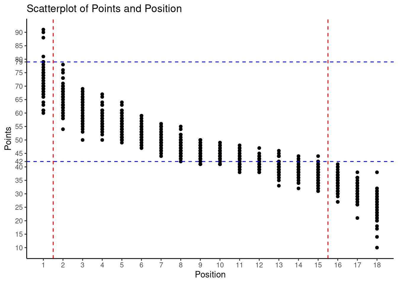
Make a scatterplot with points on the y-axis and position on the x-axis. Additionally, only consider seasons with 18 teams and add lines that make clear how many points you needed to be placed in between rank 2 and 15.
Remove all objects from the environment except dfb and liga.
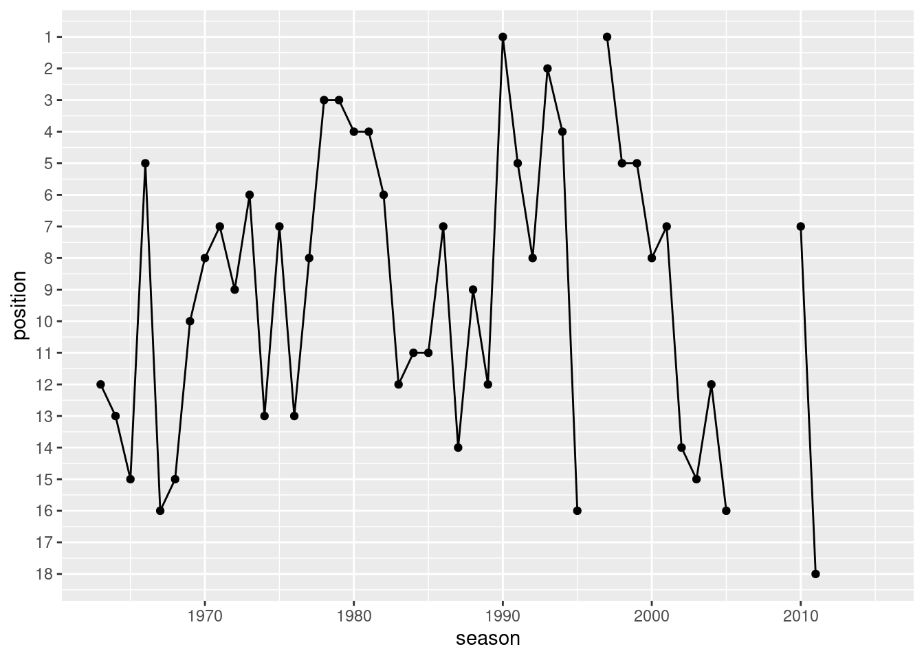
In Figure Figure 9.2, the ranking history of 1. FC Kaiserslautern is shown. Replicate that plot.
Installing package into '/home/sthu/R/x86_64-pc-linux-gnu-library/4.5'
(as 'lib' is unspecified)
bundesligR installed
Figure 9.2: Ranking history: 1. FC Kaiserslautern
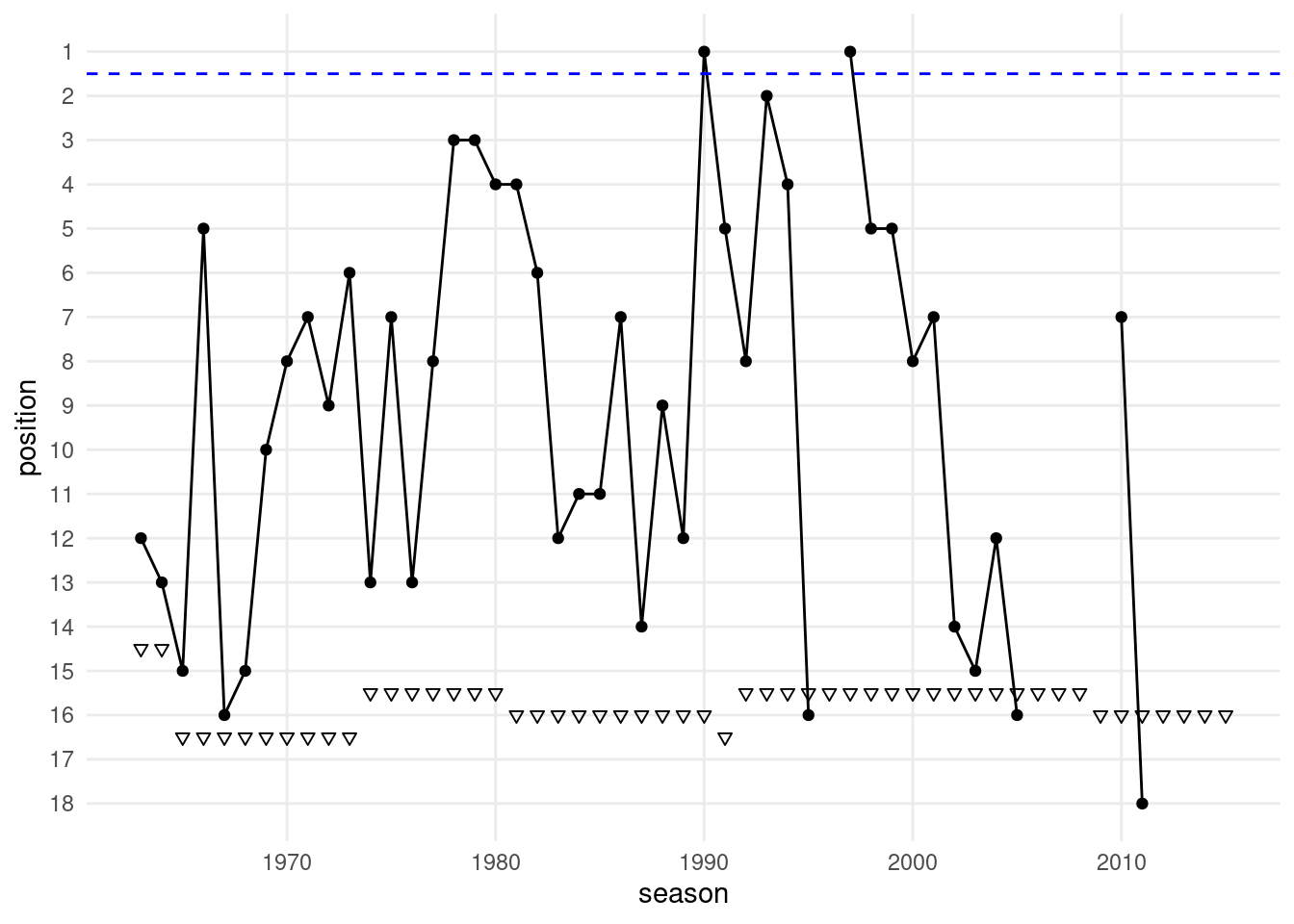
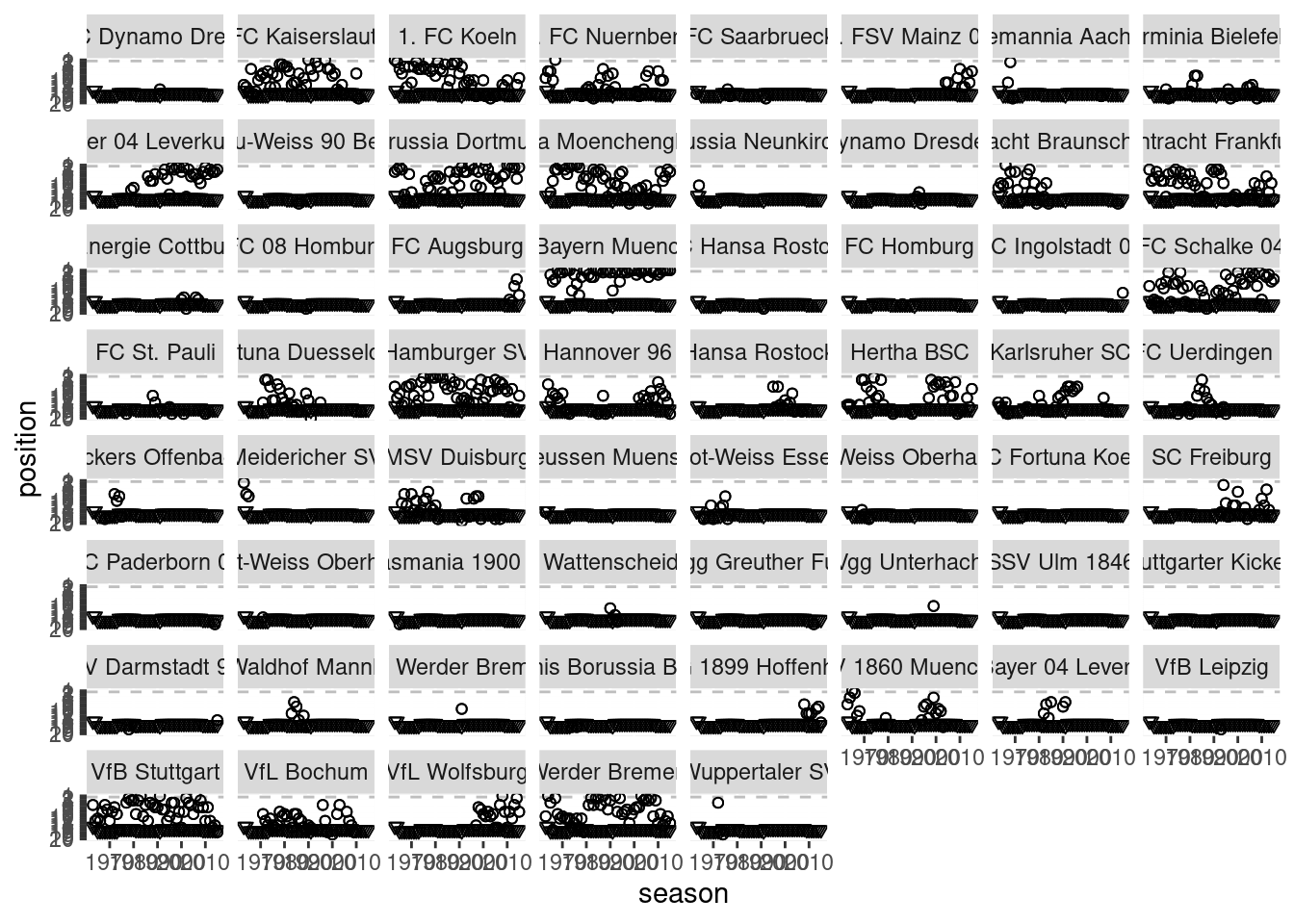
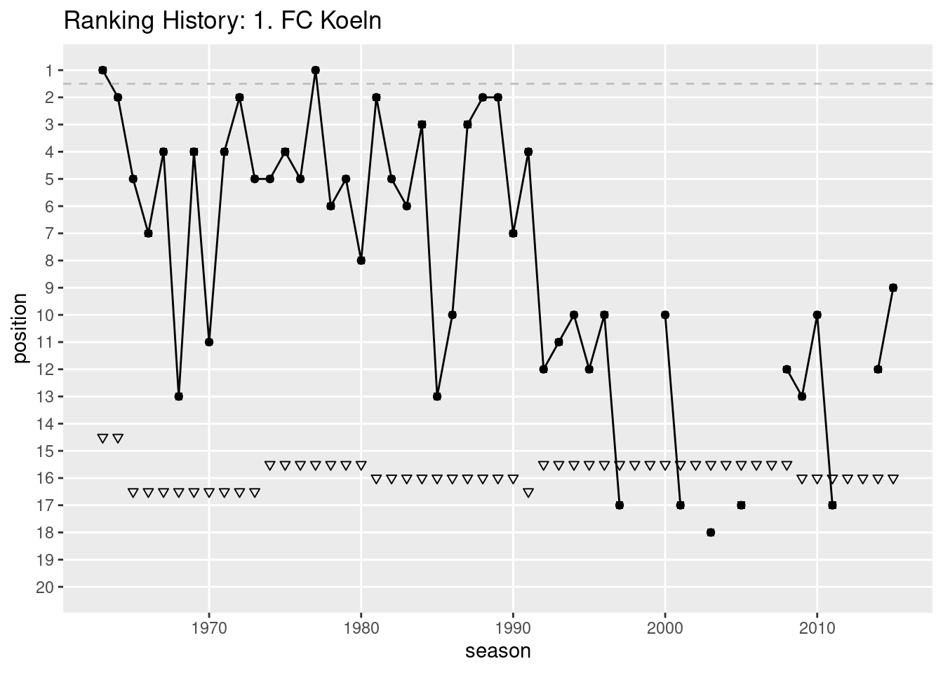
In Figure Figure 9.3, I made the graph a bit nicer. Can you spot all differences and can you guess what the dashed line and the triangles mean? How could the visualization be improved further? Replicate the plot.
Figure 9.3: Ranking history: 1. FC Köln
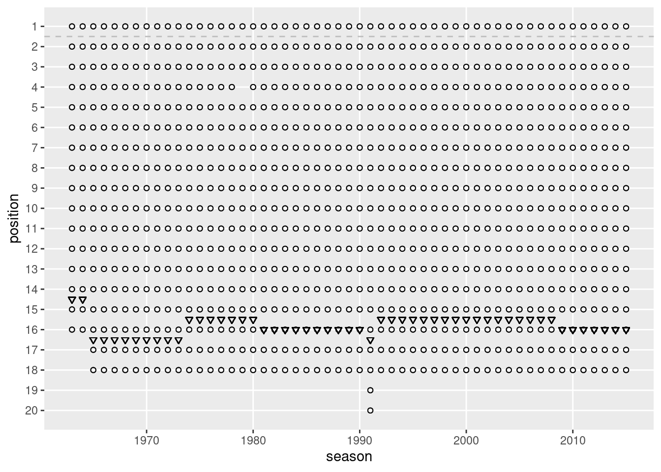
Try to make the ranking history for each club ever played the league and export the graph as a png file.
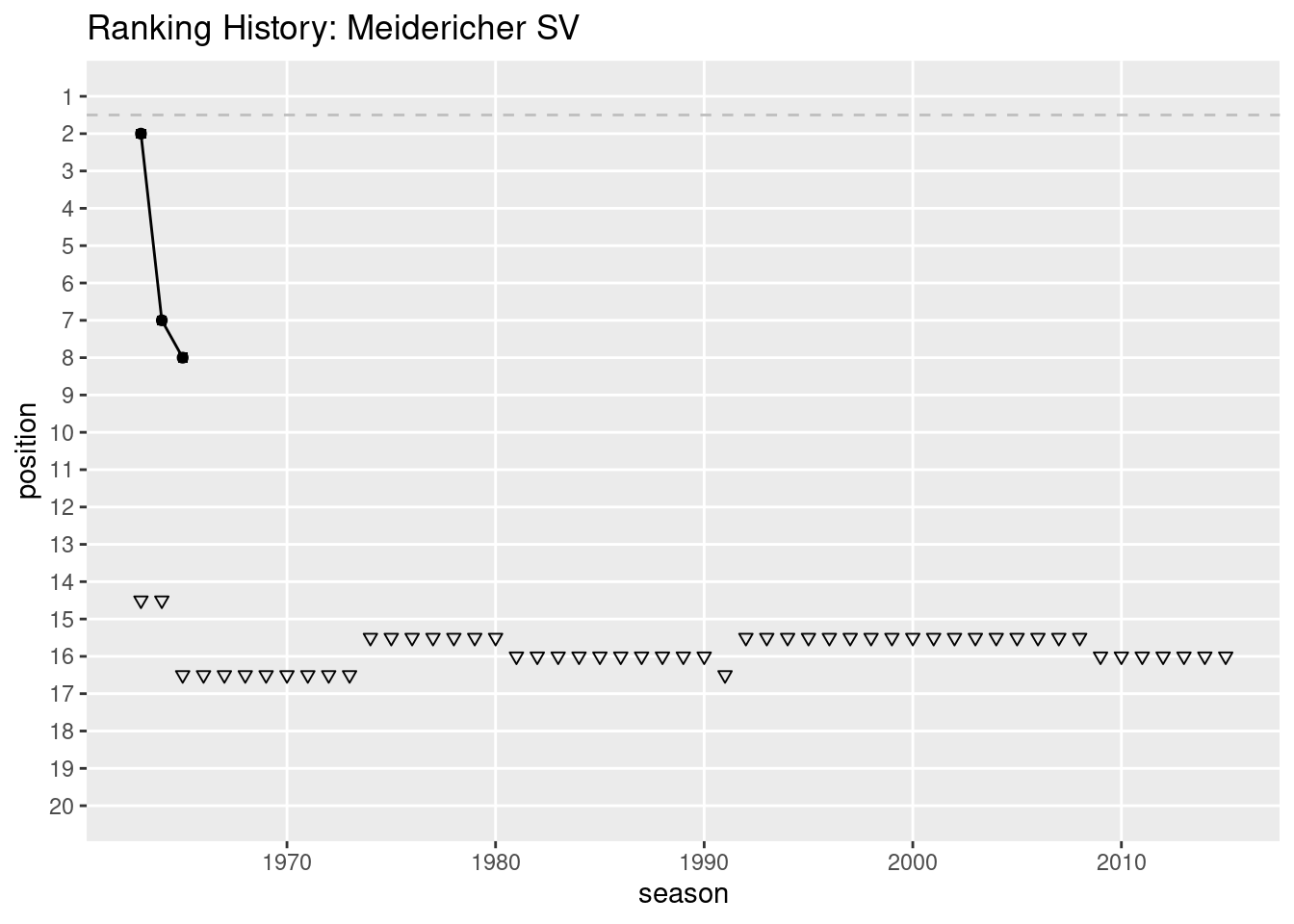
# In dfb.R I analyze German soccer results# set working directory# setwd("~/Dropbox/hsf/23-ws/dsda/scripts")# clear environmentrm(list =ls())# (Install and) load packagagesif (!require(pacman)) install.packages("pacman")pacman::p_load( bundesligR, tidyverse)# Read in the data as tibbleliga <-as_tibble(bundesligR)# --------------------------------------# !!! ERRORS / ISSUES:# "Borussia Moenchengladbach" is also entitled "Bor. Moenchengladbach"!# Leverkusen is falsly entitled "SV Bayer 04 Leverkusen"# Uerdingen has changed its name several times# Stuttgarter Kickers are named differently# How often is "Bor. Moenchengladbach" in the data?sum(liga$Team =="Bor. Moenchengladbach")# show the entriesliga |>filter(Team =="Bor. Moenchengladbach")# Replace "Bor. Moenchengladbach" with "Borussia Moenchengladbach"liga <- liga |>mutate(Team =ifelse(Team =="Bor. Moenchengladbach","Borussia Moenchengladbach", Team )) |>mutate(Team =ifelse(Team =="SV Bayer 04 Leverkusen","TSV Bayer 04 Leverkusen", Team )) |>mutate(Team =ifelse(Team =="FC Bayer 05 Uerdingen"| Team =="Bayer 05 Uerdingen","KFC Uerdingen 05", Team )) |>mutate(Team =ifelse(Team =="SV Stuttgarter Kickers","Stuttgarter Kickers", Team ))# ------------------------------------# Check for the data classclass(liga)# view dataview(liga)# Glimpse on the dataglimpse(liga)# first and last observationshead(liga)tail(liga)# summary statisticssummary(liga)# How many teams have played in the league over the years?table(liga$Season)# Which teams have played Bundesligaunique(liga$Team)# How many teams have played Bundesligan_distinct(liga$Team)# How often has each team played in the Bundesligatable(liga$Team)# summary of variable Season onlysummary(liga$Season)# summary of numeric of variables (Team is a character)liga |>select(Season, Position, Played, W, D, L, GF, GA, GD, Points, Pts_pre_95) |>summary()# shorter alternativeliga |>select(Season, Position, Played:Pts_pre_95) |>summary()# shortest alternativeliga |>select(-Team) |>filter(Season ==1999| Season ==2010) |>summary()# Most points ever received by a teamliga |>filter(Points ==max(Points))# Show only the team nameliga |>filter(Points ==max(Points)) |>select(Team) |>print()# remove the variable `Pts_pre_95` from the dataliga_post95 <- liga |>select(-Pts_pre_95)# rename W, D, and L to Win, Draw, and Loss# additionally rename GF, GA, GD to Goals_shot, Goals_received, Goal_differenceliga_longnames <- liga |>rename(Win = W, Draw = D, Loss = L) |>rename(Goals_shot = GF, Goals_received = GA, Goal_difference = GD)# Remove the variable `Pts_pre_95` from `liga`# additionally remove all observations before the year 1996liga_no3point <- liga |>select(-Pts_pre_95) |>filter(Season >=1996)# Remove the objects liga_post95, liga_longnames, and liga_no3point from the environmentrm(liga_post95, liga_longnames, liga_no3point)# Rename all variables of `liga`to lower cases and store it as `dfb`dfb <- liga |>rename_all(tolower)# Show the winner and the runner up after 2010# additionally show the pointsdfb |>filter(season >2010) |>group_by(season) |>arrange(desc(points)) |>slice_head(n =2) |>select(team, points, position)# Create a variable that counts how often a team was ranked firstdfb <- dfb |>group_by(team) |>mutate(meister_count =sum(position ==1))# How often has each team played in the Bundesligatable(liga$Team)# Make a rankingdfb |>group_by(team) |>summarise(appearances =n_distinct(season)) |>arrange(desc(appearances)) |>print(n =Inf)# Add a variable to `dfb` that contains the number of appearances of a team in the leaguedfb <- dfb |>group_by(team) |>mutate(appearances =n_distinct(season))# create a number that indicates how often a team has played Bundesliga in a given yeardfb <- dfb |>arrange(team, season) |>group_by(team) |>mutate(team_in_liga_count =row_number())# Make a ranking with the number of titles of all teams that ever won the leaguedfb |>filter(team_in_liga_count ==1) |>filter(meister_count !=0) |>arrange(desc(meister_count)) |>select(meister_count, team)# Create a numeric identifying variable for each teamdfb_teamid <- dfb |>mutate(team_id =as.numeric(factor(team)))# When a team is in the league, what is the probability that it wins the leaguedfb |>filter(team_in_liga_count ==1) |>mutate(prob_win = meister_count / appearances) |>filter(prob_win >0) |>arrange(desc(prob_win)) |>select(meister_count, prob_win, team)# make a scatterplot with points on the y-axis and position on the x-axisggplot(dfb, aes(x = position, y = points)) +geom_point()# Make a scatterplot with points on the y-axis and position on the x-axis.# Additionally, only consider seasons with 18 teams and# add lines that make clear how many points you needed to be placed# in between rank 2 and 15.dfb_18 <- dfb |>group_by(season) |>mutate(teams_in_league =n_distinct(team)) |>filter(teams_in_league ==18)h_1 <- dfb_18 |>filter(position ==16) |>mutate(ma =max(points))max_points_rank_16 <-max(h_1$ma) +1h_2 <- dfb_18 |>filter(position ==2) |>mutate(mb =max(points))min_points_rank_2 <-max(h_2$mb) +1dfb_18 <- dfb_18 |>mutate(season_category =case_when( season <1970~1,between(season, 1970, 1979) ~2,between(season, 1980, 1989) ~3,between(season, 1990, 1999) ~4,between(season, 2000, 2009) ~5,between(season, 2010, 2019) ~6,TRUE~7# Adjust this line based on the actual range of your data ))ggplot(dfb_18, aes(x = position, y = points)) +geom_point() +labs(title ="Scatterplot of Points and Position",x ="Position",y ="Points" ) +geom_vline(xintercept =c(1.5, 15.5), linetype ="dashed", color ="red") +geom_hline(yintercept = max_points_rank_16, linetype ="dashed", color ="blue") +geom_hline(yintercept = min_points_rank_2, linetype ="dashed", color ="blue") +scale_y_continuous(breaks =c(min_points_rank_2, max_points_rank_16, seq(0, max(dfb_18$points), by =5))) +scale_x_continuous(breaks =c(seq(0, max(dfb_18$points), by =1))) +theme_classic()# Remove all objects except liga and dfbrm(list =setdiff(ls(), c("liga", "dfb")))# Rank "1. FC Kaiserslautern" over timedfb_bal <- dfb |>select(season, team, position) |>as_tibble() |>complete(season, team)table(dfb_bal$team)dfb_fck <- dfb_bal |>filter(team =="1. FC Kaiserslautern")ggplot(dfb_fck, aes(x = season, y = position)) +geom_point() +geom_line() +scale_y_reverse(breaks =seq(1, 18, by =1))# Make the plot nice# consider different rules for having to leave the league:dfb_fck <- dfb_fck |>mutate(godown =ifelse(season <=1964, 14.5, NA)) |>mutate(godown =ifelse(season >1964& season <=1973, 16.5, godown)) |>mutate(godown =ifelse(season >1973& season <=1980, 15.5, godown)) |>mutate(godown =ifelse(season >1980& season <=1990, 16, godown)) |>mutate(godown =ifelse(season ==1991, 16.5, godown)) |>mutate(godown =ifelse(season >1991& season <=2008, 15.5, godown)) |>mutate(godown =ifelse(season >2008, 16, godown))ggplot(dfb_fck, aes(x = season)) +geom_point(aes(y = position)) +geom_line(aes(y = position)) +geom_point(aes(y = godown), shape =25) +scale_y_reverse(breaks =seq(1, 18, by =1)) +theme_minimal() +theme(panel.grid.minor =element_blank()) +geom_hline(yintercept =1.5, linetype ="dashed", color ="blue")dfb_bal <- dfb_bal |>mutate(godown =ifelse(season <=1964, 14.5, NA)) |>mutate(godown =ifelse(season >1964& season <=1973, 16.5, godown)) |>mutate(godown =ifelse(season >1973& season <=1980, 15.5, godown)) |>mutate(godown =ifelse(season >1980& season <=1990, 16, godown)) |>mutate(godown =ifelse(season ==1991, 16.5, godown)) |>mutate(godown =ifelse(season >1991& season <=2008, 15.5, godown)) |>mutate(godown =ifelse(season >2008, 16, godown)) |>mutate(inliga =ifelse(is.na(position), 0, 1))rank_plot <-ggplot(dfb_bal, aes(x = season)) +geom_point(aes(y = position), shape =1) +# geom_line(aes(y = position)) +geom_point(aes(y = godown), shape =25) +scale_y_reverse(breaks =seq(1, 20, by =1), limits =c(20, 1)) +xlim(1963, 2015) +theme(panel.grid.minor =element_blank()) +geom_hline(yintercept =1.5, linetype ="dashed", color ="gray") +geom_point(aes(y = position), shape =1)rank_plot# !--> in 1979 is a gap! Error?# No. Reason: two clubs shared the third place.rank_plot +facet_wrap(~team)# Create "test" directory if it doesn't already existif (!dir.exists("test")) {dir.create("test")}plots <-list()for (club inunique(dfb_bal$team)) { dfb_subset <-subset(dfb_bal, team == club) p <-ggplot(dfb_subset, aes(x = season)) +geom_point(aes(y = position), shape =15) +geom_line(aes(y = position)) +geom_point(aes(y = godown), shape =25) +scale_y_reverse(breaks =seq(1, 20, by =1), limits =c(20, 1)) +xlim(1963, 2015) +theme(panel.grid.minor =element_blank()) +geom_hline(yintercept =1.5, linetype ="dashed", color ="gray") +geom_point(aes(y = position), shape =1) +labs(title =paste("Ranking History:", club))ggsave(filename =paste("test/r_", club, ".png", sep ="")) plots[[club]] <- p}print(plots$`Meidericher SV`)print(plots$`1. FC Koeln`)# unload packagessuppressMessages(pacman::p_unload( bundesligR, tidyverse))# Remove the "test" directory and its contents after saving all graphsunlink("test", recursive =TRUE)
Output of the R script
# In dfb.R I analyze German soccer results# set working directory# setwd("~/Dropbox/hsf/23-ws/dsda/scripts")# clear environmentrm(list =ls())# (Install and) load packagagesif (!require(pacman)) install.packages("pacman")pacman::p_load( bundesligR, tidyverse)# Read in the data as tibbleliga <-as_tibble(bundesligR)# --------------------------------------# !!! ERRORS / ISSUES:# "Borussia Moenchengladbach" is also entitled "Bor. Moenchengladbach"!# Leverkusen is falsly entitled "SV Bayer 04 Leverkusen"# Uerdingen has changed its name several times# Stuttgarter Kickers are named differently# How often is "Bor. Moenchengladbach" in the data?sum(liga$Team =="Bor. Moenchengladbach")
[1] 2
# show the entriesliga |>filter(Team =="Bor. Moenchengladbach")
# A tibble: 2 × 12
Season Position Team Played W D L GF GA GD Points
<dbl> <dbl> <chr> <dbl> <dbl> <dbl> <dbl> <dbl> <dbl> <dbl> <dbl>
1 1989 15 Bor. Moench… 34 11 8 15 37 45 -8 41
2 1976 1 Bor. Moench… 34 17 10 7 58 34 24 61
# ℹ 1 more variable: Pts_pre_95 <dbl>
# Replace "Bor. Moenchengladbach" with "Borussia Moenchengladbach"liga <- liga |>mutate(Team =ifelse(Team =="Bor. Moenchengladbach","Borussia Moenchengladbach", Team )) |>mutate(Team =ifelse(Team =="SV Bayer 04 Leverkusen","TSV Bayer 04 Leverkusen", Team )) |>mutate(Team =ifelse(Team =="FC Bayer 05 Uerdingen"| Team =="Bayer 05 Uerdingen","KFC Uerdingen 05", Team )) |>mutate(Team =ifelse(Team =="SV Stuttgarter Kickers","Stuttgarter Kickers", Team ))# ------------------------------------# Check for the data classclass(liga)
[1] "tbl_df" "tbl" "data.frame"
# view dataview(liga)# Glimpse on the dataglimpse(liga)
# A tibble: 6 × 12
Season Position Team Played W D L GF GA GD Points
<dbl> <dbl> <chr> <dbl> <dbl> <dbl> <dbl> <dbl> <dbl> <dbl> <dbl>
1 2015 1 FC Bayern M… 34 28 4 2 80 17 63 88
2 2015 2 Borussia Do… 34 24 6 4 82 34 48 78
3 2015 3 Bayer 04 Le… 34 18 6 10 56 40 16 60
4 2015 4 Borussia Mo… 34 17 4 13 67 50 17 55
5 2015 5 FC Schalke … 34 15 7 12 51 49 2 52
6 2015 6 1. FSV Main… 34 14 8 12 46 42 4 50
# ℹ 1 more variable: Pts_pre_95 <dbl>
tail(liga)
# A tibble: 6 × 12
Season Position Team Played W D L GF GA GD Points
<dbl> <dbl> <chr> <dbl> <dbl> <dbl> <dbl> <dbl> <dbl> <dbl> <dbl>
1 1963 11 Eintracht B… 30 11 6 13 36 49 -13 39
2 1963 12 1. FC Kaise… 30 10 6 14 48 69 -21 36
3 1963 13 Karlsruher … 30 8 8 14 42 55 -13 32
4 1963 14 Hertha BSC 30 9 6 15 45 65 -20 33
5 1963 15 Preussen Mu… 30 7 9 14 34 52 -18 30
6 1963 16 1. FC Saarb… 30 6 5 19 44 72 -28 23
# ℹ 1 more variable: Pts_pre_95 <dbl>
# summary statisticssummary(liga)
Season Position Team Played
Min. :1963 Min. : 1.000 Length:952 Min. :30.00
1st Qu.:1976 1st Qu.: 5.000 Class :character 1st Qu.:34.00
Median :1989 Median : 9.000 Mode :character Median :34.00
Mean :1989 Mean : 9.486 Mean :33.95
3rd Qu.:2002 3rd Qu.:14.000 3rd Qu.:34.00
Max. :2015 Max. :20.000 Max. :38.00
W D L GF
Min. : 2.00 Min. : 2.000 Min. : 1.00 Min. : 15.00
1st Qu.: 9.75 1st Qu.: 7.000 1st Qu.:10.00 1st Qu.: 42.00
Median :12.00 Median : 9.000 Median :13.00 Median : 50.00
Mean :12.61 Mean : 8.733 Mean :12.61 Mean : 52.01
3rd Qu.:15.00 3rd Qu.:11.000 3rd Qu.:15.00 3rd Qu.: 61.00
Max. :29.00 Max. :18.000 Max. :28.00 Max. :101.00
GA GD Points Pts_pre_95
Min. :10.0 Min. :-60.0000 Min. :10.00 Min. : 8.00
1st Qu.:43.0 1st Qu.:-13.0000 1st Qu.:38.00 1st Qu.:29.00
Median :51.0 Median : -2.0000 Median :44.00 Median :33.00
Mean :51.7 Mean : 0.3015 Mean :46.56 Mean :33.95
3rd Qu.:60.0 3rd Qu.: 13.0000 3rd Qu.:55.00 3rd Qu.:39.00
Max. :93.0 Max. : 80.0000 Max. :91.00 Max. :62.00
# How many teams have played in the league over the years?table(liga$Season)
# How many teams have played Bundesligan_distinct(liga$Team)
[1] 61
# How often has each team played in the Bundesligatable(liga$Team)
1. FC Dynamo Dresden 1. FC Kaiserslautern 1. FC Koeln
1 44 45
1. FC Nuernberg 1. FC Saarbruecken 1. FSV Mainz 05
32 5 10
Alemannia Aachen Arminia Bielefeld Bayer 04 Leverkusen
4 17 30
Blau-Weiss 90 Berlin Borussia Dortmund Borussia Moenchengladbach
1 49 48
Borussia Neunkirchen Dynamo Dresden Eintracht Braunschweig
3 3 21
Eintracht Frankfurt Energie Cottbus FC 08 Homburg
47 6 2
FC Augsburg FC Bayern Muenchen FC Hansa Rostock
5 51 1
FC Homburg FC Ingolstadt 04 FC Schalke 04
1 1 48
FC St. Pauli Fortuna Duesseldorf Hamburger SV
8 23 53
Hannover 96 Hansa Rostock Hertha BSC
28 11 33
Karlsruher SC KFC Uerdingen 05 Kickers Offenbach
24 14 7
Meidericher SV MSV Duisburg Preussen Muenster
3 25 1
Rot-Weiss Essen Rot-Weiss Oberhausen SC Fortuna Koeln
7 3 1
SC Freiburg SC Paderborn 07 SC Rot-Weiss Oberhausen
16 1 1
SC Tasmania 1900 Berlin SG Wattenscheid 09 SpVgg Greuther Fuerth
1 4 1
SpVgg Unterhaching SSV Ulm 1846 Stuttgarter Kickers
2 1 2
SV Darmstadt 98 SV Waldhof Mannheim SV Werder Bremen
3 7 1
Tennis Borussia Berlin TSG 1899 Hoffenheim TSV 1860 Muenchen
2 8 20
TSV Bayer 04 Leverkusen VfB Leipzig VfB Stuttgart
7 1 51
VfL Bochum VfL Wolfsburg Werder Bremen
34 19 51
Wuppertaler SV
3
# summary of variable Season onlysummary(liga$Season)
Min. 1st Qu. Median Mean 3rd Qu. Max.
1963 1976 1989 1989 2002 2015
# summary of numeric of variables (Team is a character)liga |>select(Season, Position, Played, W, D, L, GF, GA, GD, Points, Pts_pre_95) |>summary()
Season Position Played W
Min. :1963 Min. : 1.000 Min. :30.00 Min. : 2.00
1st Qu.:1976 1st Qu.: 5.000 1st Qu.:34.00 1st Qu.: 9.75
Median :1989 Median : 9.000 Median :34.00 Median :12.00
Mean :1989 Mean : 9.486 Mean :33.95 Mean :12.61
3rd Qu.:2002 3rd Qu.:14.000 3rd Qu.:34.00 3rd Qu.:15.00
Max. :2015 Max. :20.000 Max. :38.00 Max. :29.00
D L GF GA
Min. : 2.000 Min. : 1.00 Min. : 15.00 Min. :10.0
1st Qu.: 7.000 1st Qu.:10.00 1st Qu.: 42.00 1st Qu.:43.0
Median : 9.000 Median :13.00 Median : 50.00 Median :51.0
Mean : 8.733 Mean :12.61 Mean : 52.01 Mean :51.7
3rd Qu.:11.000 3rd Qu.:15.00 3rd Qu.: 61.00 3rd Qu.:60.0
Max. :18.000 Max. :28.00 Max. :101.00 Max. :93.0
GD Points Pts_pre_95
Min. :-60.0000 Min. :10.00 Min. : 8.00
1st Qu.:-13.0000 1st Qu.:38.00 1st Qu.:29.00
Median : -2.0000 Median :44.00 Median :33.00
Mean : 0.3015 Mean :46.56 Mean :33.95
3rd Qu.: 13.0000 3rd Qu.:55.00 3rd Qu.:39.00
Max. : 80.0000 Max. :91.00 Max. :62.00
# shortest alternativeliga |>select(-Team) |>filter(Season ==1999| Season ==2010) |>summary()
Season Position Played W D
Min. :1999 Min. : 1.0 Min. :34 Min. : 4.00 Min. : 3.000
1st Qu.:1999 1st Qu.: 5.0 1st Qu.:34 1st Qu.: 9.75 1st Qu.: 6.000
Median :2004 Median : 9.5 Median :34 Median :12.00 Median : 8.000
Mean :2004 Mean : 9.5 Mean :34 Mean :12.83 Mean : 8.333
3rd Qu.:2010 3rd Qu.:14.0 3rd Qu.:34 3rd Qu.:14.25 3rd Qu.:10.250
Max. :2010 Max. :18.0 Max. :34 Max. :23.00 Max. :15.000
L GF GA GD
Min. : 3.00 Min. :31.00 Min. :22.00 Min. :-34.00
1st Qu.:10.75 1st Qu.:41.00 1st Qu.:44.00 1st Qu.:-10.25
Median :13.00 Median :47.00 Median :48.50 Median : -3.00
Mean :12.83 Mean :49.42 Mean :49.42 Mean : 0.00
3rd Qu.:16.00 3rd Qu.:54.25 3rd Qu.:59.00 3rd Qu.: 4.75
Max. :21.00 Max. :81.00 Max. :71.00 Max. : 45.00
Points Pts_pre_95
Min. :22.00 Min. :18.00
1st Qu.:39.75 1st Qu.:29.75
Median :44.00 Median :32.00
Mean :46.83 Mean :34.00
3rd Qu.:50.75 3rd Qu.:37.50
Max. :75.00 Max. :52.00
# Most points ever received by a teamliga |>filter(Points ==max(Points))
# A tibble: 1 × 12
Season Position Team Played W D L GF GA GD Points
<dbl> <dbl> <chr> <dbl> <dbl> <dbl> <dbl> <dbl> <dbl> <dbl> <dbl>
1 2012 1 FC Bayern M… 34 29 4 1 98 18 80 91
# ℹ 1 more variable: Pts_pre_95 <dbl>
# Show only the team nameliga |>filter(Points ==max(Points)) |>select(Team) |>print()
# A tibble: 1 × 1
Team
<chr>
1 FC Bayern Muenchen
# remove the variable `Pts_pre_95` from the dataliga_post95 <- liga |>select(-Pts_pre_95)# rename W, D, and L to Win, Draw, and Loss# additionally rename GF, GA, GD to Goals_shot, Goals_received, Goal_differenceliga_longnames <- liga |>rename(Win = W, Draw = D, Loss = L) |>rename(Goals_shot = GF, Goals_received = GA, Goal_difference = GD)# Remove the variable `Pts_pre_95` from `liga`# additionally remove all observations before the year 1996liga_no3point <- liga |>select(-Pts_pre_95) |>filter(Season >=1996)# Remove the objects liga_post95, liga_longnames, and liga_no3point from the environmentrm(liga_post95, liga_longnames, liga_no3point)# Rename all variables of `liga`to lower cases and store it as `dfb`dfb <- liga |>rename_all(tolower)# Show the winner and the runner up after 2010# additionally show the pointsdfb |>filter(season >2010) |>group_by(season) |>arrange(desc(points)) |>slice_head(n =2) |>select(team, points, position)
# A tibble: 10 × 4
# Groups: season [5]
season team points position
<dbl> <chr> <dbl> <dbl>
1 2011 Borussia Dortmund 81 1
2 2011 FC Bayern Muenchen 73 2
3 2012 FC Bayern Muenchen 91 1
4 2012 Borussia Dortmund 66 2
5 2013 FC Bayern Muenchen 90 1
6 2013 Borussia Dortmund 71 2
7 2014 FC Bayern Muenchen 79 1
8 2014 VfL Wolfsburg 69 2
9 2015 FC Bayern Muenchen 88 1
10 2015 Borussia Dortmund 78 2
# Create a variable that counts how often a team was ranked firstdfb <- dfb |>group_by(team) |>mutate(meister_count =sum(position ==1))# How often has each team played in the Bundesligatable(liga$Team)
1. FC Dynamo Dresden 1. FC Kaiserslautern 1. FC Koeln
1 44 45
1. FC Nuernberg 1. FC Saarbruecken 1. FSV Mainz 05
32 5 10
Alemannia Aachen Arminia Bielefeld Bayer 04 Leverkusen
4 17 30
Blau-Weiss 90 Berlin Borussia Dortmund Borussia Moenchengladbach
1 49 48
Borussia Neunkirchen Dynamo Dresden Eintracht Braunschweig
3 3 21
Eintracht Frankfurt Energie Cottbus FC 08 Homburg
47 6 2
FC Augsburg FC Bayern Muenchen FC Hansa Rostock
5 51 1
FC Homburg FC Ingolstadt 04 FC Schalke 04
1 1 48
FC St. Pauli Fortuna Duesseldorf Hamburger SV
8 23 53
Hannover 96 Hansa Rostock Hertha BSC
28 11 33
Karlsruher SC KFC Uerdingen 05 Kickers Offenbach
24 14 7
Meidericher SV MSV Duisburg Preussen Muenster
3 25 1
Rot-Weiss Essen Rot-Weiss Oberhausen SC Fortuna Koeln
7 3 1
SC Freiburg SC Paderborn 07 SC Rot-Weiss Oberhausen
16 1 1
SC Tasmania 1900 Berlin SG Wattenscheid 09 SpVgg Greuther Fuerth
1 4 1
SpVgg Unterhaching SSV Ulm 1846 Stuttgarter Kickers
2 1 2
SV Darmstadt 98 SV Waldhof Mannheim SV Werder Bremen
3 7 1
Tennis Borussia Berlin TSG 1899 Hoffenheim TSV 1860 Muenchen
2 8 20
TSV Bayer 04 Leverkusen VfB Leipzig VfB Stuttgart
7 1 51
VfL Bochum VfL Wolfsburg Werder Bremen
34 19 51
Wuppertaler SV
3
# Make a rankingdfb |>group_by(team) |>summarise(appearances =n_distinct(season)) |>arrange(desc(appearances)) |>print(n =Inf)
# Add a variable to `dfb` that contains the number of appearances of a team in the leaguedfb <- dfb |>group_by(team) |>mutate(appearances =n_distinct(season))# create a number that indicates how often a team has played Bundesliga in a given yeardfb <- dfb |>arrange(team, season) |>group_by(team) |>mutate(team_in_liga_count =row_number())# Make a ranking with the number of titles of all teams that ever won the leaguedfb |>filter(team_in_liga_count ==1) |>filter(meister_count !=0) |>arrange(desc(meister_count)) |>select(meister_count, team)
# A tibble: 12 × 2
# Groups: team [12]
meister_count team
<int> <chr>
1 25 FC Bayern Muenchen
2 5 Borussia Dortmund
3 5 Borussia Moenchengladbach
4 4 Werder Bremen
5 3 Hamburger SV
6 3 VfB Stuttgart
7 2 1. FC Kaiserslautern
8 2 1. FC Koeln
9 1 1. FC Nuernberg
10 1 Eintracht Braunschweig
11 1 TSV 1860 Muenchen
12 1 VfL Wolfsburg
# Create a numeric identifying variable for each teamdfb_teamid <- dfb |>mutate(team_id =as.numeric(factor(team)))# When a team is in the league, what is the probability that it wins the leaguedfb |>filter(team_in_liga_count ==1) |>mutate(prob_win = meister_count / appearances) |>filter(prob_win >0) |>arrange(desc(prob_win)) |>select(meister_count, prob_win, team)
# make a scatterplot with points on the y-axis and position on the x-axisggplot(dfb, aes(x = position, y = points)) +geom_point()
# Make a scatterplot with points on the y-axis and position on the x-axis.# Additionally, only consider seasons with 18 teams and# add lines that make clear how many points you needed to be placed# in between rank 2 and 15.dfb_18 <- dfb |>group_by(season) |>mutate(teams_in_league =n_distinct(team)) |>filter(teams_in_league ==18)h_1 <- dfb_18 |>filter(position ==16) |>mutate(ma =max(points))max_points_rank_16 <-max(h_1$ma) +1h_2 <- dfb_18 |>filter(position ==2) |>mutate(mb =max(points))min_points_rank_2 <-max(h_2$mb) +1dfb_18 <- dfb_18 |>mutate(season_category =case_when( season <1970~1,between(season, 1970, 1979) ~2,between(season, 1980, 1989) ~3,between(season, 1990, 1999) ~4,between(season, 2000, 2009) ~5,between(season, 2010, 2019) ~6,TRUE~7# Adjust this line based on the actual range of your data ))ggplot(dfb_18, aes(x = position, y = points)) +geom_point() +labs(title ="Scatterplot of Points and Position",x ="Position",y ="Points" ) +geom_vline(xintercept =c(1.5, 15.5), linetype ="dashed", color ="red") +geom_hline(yintercept = max_points_rank_16, linetype ="dashed", color ="blue") +geom_hline(yintercept = min_points_rank_2, linetype ="dashed", color ="blue") +scale_y_continuous(breaks =c(min_points_rank_2, max_points_rank_16, seq(0, max(dfb_18$points), by =5))) +scale_x_continuous(breaks =c(seq(0, max(dfb_18$points), by =1))) +theme_classic()
# Remove all objects except liga and dfbrm(list =setdiff(ls(), c("liga", "dfb")))# Rank "1. FC Kaiserslautern" over timedfb_bal <- dfb |>select(season, team, position) |>as_tibble() |>complete(season, team)table(dfb_bal$team)
1. FC Dynamo Dresden 1. FC Kaiserslautern 1. FC Koeln
53 53 53
1. FC Nuernberg 1. FC Saarbruecken 1. FSV Mainz 05
53 53 53
Alemannia Aachen Arminia Bielefeld Bayer 04 Leverkusen
53 53 53
Blau-Weiss 90 Berlin Borussia Dortmund Borussia Moenchengladbach
53 53 53
Borussia Neunkirchen Dynamo Dresden Eintracht Braunschweig
53 53 53
Eintracht Frankfurt Energie Cottbus FC 08 Homburg
53 53 53
FC Augsburg FC Bayern Muenchen FC Hansa Rostock
53 53 53
FC Homburg FC Ingolstadt 04 FC Schalke 04
53 53 53
FC St. Pauli Fortuna Duesseldorf Hamburger SV
53 53 53
Hannover 96 Hansa Rostock Hertha BSC
53 53 53
Karlsruher SC KFC Uerdingen 05 Kickers Offenbach
53 53 53
Meidericher SV MSV Duisburg Preussen Muenster
53 53 53
Rot-Weiss Essen Rot-Weiss Oberhausen SC Fortuna Koeln
53 53 53
SC Freiburg SC Paderborn 07 SC Rot-Weiss Oberhausen
53 53 53
SC Tasmania 1900 Berlin SG Wattenscheid 09 SpVgg Greuther Fuerth
53 53 53
SpVgg Unterhaching SSV Ulm 1846 Stuttgarter Kickers
53 53 53
SV Darmstadt 98 SV Waldhof Mannheim SV Werder Bremen
53 53 53
Tennis Borussia Berlin TSG 1899 Hoffenheim TSV 1860 Muenchen
53 53 53
TSV Bayer 04 Leverkusen VfB Leipzig VfB Stuttgart
53 53 53
VfL Bochum VfL Wolfsburg Werder Bremen
53 53 53
Wuppertaler SV
53
dfb_fck <- dfb_bal |>filter(team =="1. FC Kaiserslautern")ggplot(dfb_fck, aes(x = season, y = position)) +geom_point() +geom_line() +scale_y_reverse(breaks =seq(1, 18, by =1))
# Make the plot nice# consider different rules for having to leave the league:dfb_fck <- dfb_fck |>mutate(godown =ifelse(season <=1964, 14.5, NA)) |>mutate(godown =ifelse(season >1964& season <=1973, 16.5, godown)) |>mutate(godown =ifelse(season >1973& season <=1980, 15.5, godown)) |>mutate(godown =ifelse(season >1980& season <=1990, 16, godown)) |>mutate(godown =ifelse(season ==1991, 16.5, godown)) |>mutate(godown =ifelse(season >1991& season <=2008, 15.5, godown)) |>mutate(godown =ifelse(season >2008, 16, godown))ggplot(dfb_fck, aes(x = season)) +geom_point(aes(y = position)) +geom_line(aes(y = position)) +geom_point(aes(y = godown), shape =25) +scale_y_reverse(breaks =seq(1, 18, by =1)) +theme_minimal() +theme(panel.grid.minor =element_blank()) +geom_hline(yintercept =1.5, linetype ="dashed", color ="blue")
# unload packagessuppressMessages(pacman::p_unload( bundesligR, tidyverse))# Remove the "test" directory and its contents after saving all graphsunlink("test", recursive =TRUE)
9.16 Okun’s Law
Suppose you aim to empirically examine unemployment and GDP for Germany and France. The data set that we use in the following is ‘forest.Rdata’ and should already been known to you from the lecture.
Write down your name, matriculation number, and date.
Set your working directory.
Clear your global environment.
Install and load the following packages: ‘tidyverse’, ‘sjPlot’, and ‘ggpubr’
Download and load the data, respectively, with the following code:
If that is not working, you can also download the data from ILIAS, save it in your working directory and load it from there with:
load("forest.Rdata")
Show the first eight observations of the dataset df.
Show the last observation of the dataset df.
Which type of data do we have here (Panel, cross-section,time series, …)? Name the variable(s) that are necessary to identify the observations in the dataset.
Explain what the assignment operator in R is and what it is good for.
Write down the R code to store the number of observations and the number of variables that are in the dataset df. Name the object in which you store these numbers observations_df.
In the dataset df, rename the variable ‘country.x’ to ‘nation’ and the variable ‘date’ to ‘year’.
Explain what the pipe operator in R is and what it is good for.
For the upcoming analysis you are only interested the following variables that are part of the dataframe df: nation, year, gdp, pop, gdppc, and unemployment. Drop all other variables from the dataframe df.
Create a variable that indicates the GDP per capita (‘gdp’ divided by ‘pop’). Name the variable ‘gdp_pc’. (Hint: If you fail here, use the variable ‘gdppc’ which is already in the dataset as a replacement for ‘gdp_pc’ in the following tasks.)
For the upcoming analysis you are only interested the following countries that are part of the dataframe df: Germany and France. Drop all other countries from the dataframe df.
Create a table showing the average unemployment rate and GDP per capita for Germany and France in the given years. Use the pipe operator. (Hint: See below for how your results should look like.)
# A tibble: 2 × 3
nation `mean(unemployment)` `mean(gdppc)`
<chr> <dbl> <dbl>
1 France 9.75 34356.
2 Germany 7.22 36739.
Create a table showing the unemployment rate and GDP per capita for Germany and France in the year 2020. Use the pipe operator. (Hint: See below for how your results should look like.)
# A tibble: 2 × 3
nation `mean(unemployment)` `mean(gdppc)`
<chr> <dbl> <dbl>
1 France 8.01 35786.
2 Germany 3.81 41315.
Create a table showing the highest unemployment rate and the highest GDP per capita for Germany and France during the given period. Use the pipe operator. (Hint: See below for how your results should look like.)
# A tibble: 2 × 3
nation `max(unemployment)` `max(gdppc)`
<chr> <dbl> <dbl>
1 France 12.6 38912.
2 Germany 11.2 43329.
Calculate the standard deviation of the unemployment rate and GDP per capita for Germany and France in the given years. (Hint: See below for how your result should look like.)
# A tibble: 2 × 3
nation `sd(gdppc)` `sd(unemployment)`
<chr> <dbl> <dbl>
1 France 2940. 1.58
2 Germany 4015. 2.37
In statistics, the coefficient of variation (COV) is a standardized measure of dispersion. It is defined as the ratio of the standard deviation (\(\sigma\)) to the mean (\(\mu\)): \(COV={\frac {\sigma }{\mu }}\). Write down the R code to calculate the coefficient of variation (COV) for the unemployment rate in Germany and France. (Hint: See below for what your result should should look like.)
Write down the R code to calculate the coefficient of variation (COV) for the GDP per capita in Germany and France. (Hint: See below for what your result should should look like.)
Create a chart (bar chart, line chart, or scatter plot) that shows the unemployment rate of Germany over the available years. Label the chart ‘Germany’ with ggtitle("Germany"). Please note that you may choose any type of graphical representation. (Hint: Below you can see one of many possible examples of what your result may look like).
and 23. (This task is worth 10 points) The following chart shows the simultaneous development of the unemployment rate and GDP per capita over time for France.
Suppose you want to visualize the simultaneous evolution of the unemployment rate and GDP per capita over time for Germany as well.
Suppose further that you have found the following lines of code that create the kind of chart you are looking for.
# Datax <-c(1, 2, 3, 4, 5, 4, 7, 8, 9)y <-c(12, 16, 14, 18, 16, 13, 15, 20, 22)labels <-1970:1978# Connected scatter plot with textplot(x, y, type ="b", xlab ="Var 1", ylab ="Var 2")text(x +0.4, y +0.1, labels)
Use these lines of code and customize them to create the co-movement visualization for Germany using the available df data. The result should look something like this:
Interpret the two graphs above, which show the simultaneous evolution of the unemployment rate and GDP per capita over time for Germany and France. What are your expectations regarding the correlation between the unemployment rate and GDP per capita variables? Can you see this expectation in the figures? Discuss.
Solution
The script uses the following functions: aes, c, dim, filter, geom_line, ggplot, ggtitle, group_by, head, load, max, mean, mutate, plot, rename, sd, select, summarise, tail, text, title, url.
After loading the dataset, remove all objects except df_2022 and df_2022_error.
Reorder the data using the relocate function so that surname, name, and age appear first. Save the changed data in a tibble called df.
Sort the data according to surname, name, and age.
Make a variable named born that contains the year of birth. How is the born variable calculated?
Create a new variable named id that identifies each person by surname, name, and their birth year (born). Why is this identifier useful?
Investigate how the data is identified. Are there any duplicates? If so, can you think of strategies to identify and how to deal with these duplicates.
Unload the packages used in the script. Why is unloading packages considered good practice?
Solution
The script uses the following functions: anti_join, arrange, c, cur_group_id, desc, dim, distinct, filter, get_dupes, glimpse, group_by, head, load, max, mutate, n, paste, relocate, row_number, setdiff, summary, tail, ungroup, url.
R script
# Find duplicates# set working directory# setwd("~/Dropbox/hsf/test/initial_script")# clear environmentrm(list =ls())# load packagesif (!require(pacman)) install.packages("pacman")pacman::p_load(tidyverse, janitor, babynames, stringr)load(url("https://github.com/hubchev/courses/raw/main/dta/df_names.RData"))# Remove all objects except df_2022 and df_2022_errorrm(list =setdiff(ls(), c("df_2022_error", "df_2022")))# Re-order the data so that surname, name, and age appears first.# Save the changed data in a tibble called `df`.df <- df_2022 |>relocate(surname, name, age)# Sort the data according to surname, name, and age.df <- df |>arrange(surname, name, age)# Inspect df_2022 and df_2022_errordfdim(df)head(df)tail(df)glimpse(df)summary(df)df_2022_error# Make a variable that contains the year of birth. Name the variable `born`# and new dataframe `df`.df <- df_2022 |>mutate(born = time - age)# Make a new variable that identifies each person by surname, name,# and their birth born. Name the variable `id`.df <- df |>mutate(id =paste(surname, name, born, sep ="_"))# How many different groups do exist?df <- df |>group_by(id) |>mutate(id_num =cur_group_id()) |>ungroup()max(df$id_num)# Show groups that exist more than once.df <- df |>group_by(id) |>mutate(dup_count =row_number(),dup_sum =n() ) |>ungroup() |>arrange(id)df |>filter(dup_sum >1)df |>get_dupes(name, surname)# Make yourself familiar with the function `get_dupes()` from `janitor` package.df |>get_dupes()df |>get_dupes(surname, name)df |>get_dupes(id)df_uni <- df |>arrange() |>distinct(id, .keep_all =TRUE)df_uni_b <- df |>arrange(desc(dup_count)) |>distinct(id, .keep_all =TRUE)anti_join(df, df_uni)anti_join(df, df_uni_b)# unload packagessuppressMessages(pacman::p_unload(tidyverse, janitor, babynames, stringr))
Output of the R script
# Find duplicates# set working directory# setwd("~/Dropbox/hsf/test/initial_script")# clear environmentrm(list =ls())# load packagesif (!require(pacman)) install.packages("pacman")pacman::p_load(tidyverse, janitor, babynames, stringr)load(url("https://github.com/hubchev/courses/raw/main/dta/df_names.RData"))# Remove all objects except df_2022 and df_2022_errorrm(list =setdiff(ls(), c("df_2022_error", "df_2022")))# Re-order the data so that surname, name, and age appears first.# Save the changed data in a tibble called `df`.df <- df_2022 |>relocate(surname, name, age)# Sort the data according to surname, name, and age.df <- df |>arrange(surname, name, age)# Inspect df_2022 and df_2022_errordf
# A tibble: 1,018 × 8
surname name age sex cm time error error_desc
<chr> <chr> <dbl> <chr> <dbl> <dbl> <dbl> <chr>
1 Adams Adonnis 30 M 192 2022 0 <NA>
2 Adams Adonnis 30 M 192 2022 1 duplicate
3 Adams Aila 79 F 157 2022 0 <NA>
4 Adams Avenelle 69 F 157 2022 0 <NA>
5 Adams Brysan 39 M 192 2022 0 <NA>
6 Adams Eona 84 F 157 2022 0 <NA>
7 Adams Eveline 42 F 157 2022 0 <NA>
8 Adams Faithe 17 F 172. 2022 0 <NA>
9 Adams Ineisha 47 F 157 2022 0 <NA>
10 Adams Kloeigh 31 F 157 2022 0 <NA>
# ℹ 1,008 more rows
dim(df)
[1] 1018 8
head(df)
# A tibble: 6 × 8
surname name age sex cm time error error_desc
<chr> <chr> <dbl> <chr> <dbl> <dbl> <dbl> <chr>
1 Adams Adonnis 30 M 192 2022 0 <NA>
2 Adams Adonnis 30 M 192 2022 1 duplicate
3 Adams Aila 79 F 157 2022 0 <NA>
4 Adams Avenelle 69 F 157 2022 0 <NA>
5 Adams Brysan 39 M 192 2022 0 <NA>
6 Adams Eona 84 F 157 2022 0 <NA>
tail(df)
# A tibble: 6 × 8
surname name age sex cm time error error_desc
<chr> <chr> <dbl> <chr> <dbl> <dbl> <dbl> <chr>
1 Young Leiliana 54 F 157 2022 0 <NA>
2 Young Shamar 23 M 192 2022 0 <NA>
3 Young Tajanay 1 F 81.5 2022 0 <NA>
4 huber Stephan 186 M 41 2022 1 age/cm false, not capitalized …
5 huber Stephan NA <NA> NA 2022 1 wrong name
6 <NA> Zita 6 <NA> 110 2022 2 surname missing, sex unspecifi…
surname name age sex
Length:1018 Length:1018 Min. : 1.00 Length:1018
Class :character Class :character 1st Qu.: 21.00 Class :character
Mode :character Mode :character Median : 43.00 Mode :character
Mean : 45.75
3rd Qu.: 69.00
Max. :399.00
NA's :2
cm time error error_desc
Min. : 41.0 Min. :2022 Min. :0.00000 Length:1018
1st Qu.:157.0 1st Qu.:2022 1st Qu.:0.00000 Class :character
Median :157.0 Median :2022 Median :0.00000 Mode :character
Mean :163.2 Mean :2022 Mean :0.02456
3rd Qu.:192.0 3rd Qu.:2022 3rd Qu.:0.00000
Max. :295.0 Max. :2022 Max. :3.00000
NA's :4
df_2022_error
# A tibble: 18 × 8
sex name surname age cm time error error_desc
<chr> <chr> <chr> <dbl> <dbl> <dbl> <dbl> <chr>
1 M Savier Campbell 72 192 2022 1 duplicate
2 F Tina Adams 5 98.0 2022 1 duplicate
3 F Abery Allen 79 157 2022 1 duplicate
4 M Adonnis Adams 30 192 2022 1 duplicate
5 M Stephan Maier 41 186 2022 1 wrong surname
6 <NA> Stephan huber NA NA 2022 1 wrong name
7 M stephan Huber 186 41 2022 1 age/cm false, not capitalized…
8 M Stephan huber 186 41 2022 1 age/cm false, not capitalized…
9 M Stephan Huber 41 186 2022 1 duplicate
10 M Stephan Huber 41 NA 2022 1 duplicate, cm NA
11 F Rosa Huber 9 NA 2022 3 only age and sex given
12 <NA> Rosa Huber NA 130 2022 3 age missing, sex unspecified
13 <NA> Ignaz Huber 7 NA 2022 2 cm missing, sex unspecified
14 <NA> Zita <NA> 6 110 2022 2 surname missing, sex unspecif…
15 <NA> Alois Huber 3 295 2022 2 cm not possible, sex unspecif…
16 F Martina Huber 399 169 2022 2 age not possible
17 M Stephan Huber 41 186 2022 0 no error
18 M Stephan Huber 41 186 2022 1 duplicate
# Make a variable that contains the year of birth. Name the variable `born`# and new dataframe `df`.df <- df_2022 |>mutate(born = time - age)# Make a new variable that identifies each person by surname, name,# and their birth born. Name the variable `id`.df <- df |>mutate(id =paste(surname, name, born, sep ="_"))# How many different groups do exist?df <- df |>group_by(id) |>mutate(id_num =cur_group_id()) |>ungroup()max(df$id_num)
[1] 1011
# Show groups that exist more than once.df <- df |>group_by(id) |>mutate(dup_count =row_number(),dup_sum =n() ) |>ungroup() |>arrange(id)df |>filter(dup_sum >1)
# A tibble: 12 × 13
sex name surname age cm time error error_desc born id id_num
<chr> <chr> <chr> <dbl> <dbl> <dbl> <dbl> <chr> <dbl> <chr> <int>
1 M Adonnis Adams 30 192 2022 0 <NA> 1992 Adam… 1
2 M Adonnis Adams 30 192 2022 1 duplicate 1992 Adam… 1
3 F Tina Adams 5 98.0 2022 1 duplicate 2017 Adam… 13
4 F Tina Adams 5 98.0 2022 0 <NA> 2017 Adam… 13
5 F Abery Allen 79 157 2022 0 <NA> 1943 Alle… 15
6 F Abery Allen 79 157 2022 1 duplicate 1943 Alle… 15
7 M Savier Campbell 72 192 2022 0 <NA> 1950 Camp… 100
8 M Savier Campbell 72 192 2022 1 duplicate 1950 Camp… 100
9 M Stephan Huber 41 186 2022 1 duplicate 1981 Hube… 383
10 M Stephan Huber 41 186 2022 0 no error 1981 Hube… 383
11 M Stephan Huber 41 186 2022 1 duplicate 1981 Hube… 383
12 M Stephan Huber 41 NA 2022 1 duplicate,… 1981 Hube… 383
# ℹ 2 more variables: dup_count <int>, dup_sum <int>
df |>get_dupes(name, surname)
# A tibble: 18 × 14
name surname dupe_count sex age cm time error error_desc born id
<chr> <chr> <int> <chr> <dbl> <dbl> <dbl> <dbl> <chr> <dbl> <chr>
1 Step… Huber 4 M 41 186 2022 1 duplicate 1981 Hube…
2 Step… Huber 4 M 41 186 2022 0 no error 1981 Hube…
3 Step… Huber 4 M 41 186 2022 1 duplicate 1981 Hube…
4 Step… Huber 4 M 41 NA 2022 1 duplicate… 1981 Hube…
5 Abery Allen 2 F 79 157 2022 0 <NA> 1943 Alle…
6 Abery Allen 2 F 79 157 2022 1 duplicate 1943 Alle…
7 Adon… Adams 2 M 30 192 2022 0 <NA> 1992 Adam…
8 Adon… Adams 2 M 30 192 2022 1 duplicate 1992 Adam…
9 Merl… Miller 2 F 12 153. 2022 0 <NA> 2010 Mill…
10 Merl… Miller 2 F 2 99.9 2022 0 <NA> 2020 Mill…
11 Rosa Huber 2 F 9 NA 2022 3 only age … 2013 Hube…
12 Rosa Huber 2 <NA> NA 130 2022 3 age missi… NA Hube…
13 Savi… Campbe… 2 M 72 192 2022 0 <NA> 1950 Camp…
14 Savi… Campbe… 2 M 72 192 2022 1 duplicate 1950 Camp…
15 Step… huber 2 M 186 41 2022 1 age/cm fa… 1836 hube…
16 Step… huber 2 <NA> NA NA 2022 1 wrong name NA hube…
17 Tina Adams 2 F 5 98.0 2022 1 duplicate 2017 Adam…
18 Tina Adams 2 F 5 98.0 2022 0 <NA> 2017 Adam…
# ℹ 3 more variables: id_num <int>, dup_count <int>, dup_sum <int>
# Make yourself familiar with the function `get_dupes()` from `janitor` package.df |>get_dupes()
No variable names specified - using all columns.
No duplicate combinations found of: sex, name, surname, age, cm, time, error, error_desc, born, ... and 4 other variables
# A tibble: 0 × 14
# ℹ 14 variables: sex <chr>, name <chr>, surname <chr>, age <dbl>, cm <dbl>,
# time <dbl>, error <dbl>, error_desc <chr>, born <dbl>, id <chr>,
# id_num <int>, dup_count <int>, dup_sum <int>, dupe_count <int>
df |>get_dupes(surname, name)
# A tibble: 18 × 14
surname name dupe_count sex age cm time error error_desc born id
<chr> <chr> <int> <chr> <dbl> <dbl> <dbl> <dbl> <chr> <dbl> <chr>
1 Huber Step… 4 M 41 186 2022 1 duplicate 1981 Hube…
2 Huber Step… 4 M 41 186 2022 0 no error 1981 Hube…
3 Huber Step… 4 M 41 186 2022 1 duplicate 1981 Hube…
4 Huber Step… 4 M 41 NA 2022 1 duplicate… 1981 Hube…
5 Adams Adon… 2 M 30 192 2022 0 <NA> 1992 Adam…
6 Adams Adon… 2 M 30 192 2022 1 duplicate 1992 Adam…
7 Adams Tina 2 F 5 98.0 2022 1 duplicate 2017 Adam…
8 Adams Tina 2 F 5 98.0 2022 0 <NA> 2017 Adam…
9 Allen Abery 2 F 79 157 2022 0 <NA> 1943 Alle…
10 Allen Abery 2 F 79 157 2022 1 duplicate 1943 Alle…
11 Campbe… Savi… 2 M 72 192 2022 0 <NA> 1950 Camp…
12 Campbe… Savi… 2 M 72 192 2022 1 duplicate 1950 Camp…
13 Huber Rosa 2 F 9 NA 2022 3 only age … 2013 Hube…
14 Huber Rosa 2 <NA> NA 130 2022 3 age missi… NA Hube…
15 Miller Merl… 2 F 12 153. 2022 0 <NA> 2010 Mill…
16 Miller Merl… 2 F 2 99.9 2022 0 <NA> 2020 Mill…
17 huber Step… 2 M 186 41 2022 1 age/cm fa… 1836 hube…
18 huber Step… 2 <NA> NA NA 2022 1 wrong name NA hube…
# ℹ 3 more variables: id_num <int>, dup_count <int>, dup_sum <int>
df |>get_dupes(id)
# A tibble: 12 × 14
id dupe_count sex name surname age cm time error error_desc born
<chr> <int> <chr> <chr> <chr> <dbl> <dbl> <dbl> <dbl> <chr> <dbl>
1 Hube… 4 M Step… Huber 41 186 2022 1 duplicate 1981
2 Hube… 4 M Step… Huber 41 186 2022 0 no error 1981
3 Hube… 4 M Step… Huber 41 186 2022 1 duplicate 1981
4 Hube… 4 M Step… Huber 41 NA 2022 1 duplicate… 1981
5 Adam… 2 M Adon… Adams 30 192 2022 0 <NA> 1992
6 Adam… 2 M Adon… Adams 30 192 2022 1 duplicate 1992
7 Adam… 2 F Tina Adams 5 98.0 2022 1 duplicate 2017
8 Adam… 2 F Tina Adams 5 98.0 2022 0 <NA> 2017
9 Alle… 2 F Abery Allen 79 157 2022 0 <NA> 1943
10 Alle… 2 F Abery Allen 79 157 2022 1 duplicate 1943
11 Camp… 2 M Savi… Campbe… 72 192 2022 0 <NA> 1950
12 Camp… 2 M Savi… Campbe… 72 192 2022 1 duplicate 1950
# ℹ 3 more variables: id_num <int>, dup_count <int>, dup_sum <int>
The data under investigation includes population information for various German cities, identified by the variable stadt, spanning the years 1970, 1987, and 2010. The variable status provides details about the legislative status of the cities, and the variable state (Bundesland) indicates the state in which each respective city is situated.
Preamble
Set your working directory.
Clear your global environment.
Install and load the following packages: ‘tidyverse’, ‘haven’, and ‘janitor’.
Installing package into '/home/sthu/R/x86_64-pc-linux-gnu-library/4.5'
(as 'lib' is unspecified)
also installing the dependencies 'broom.mixed', 'pander'
jtools installed
Read in, inspect, and clean the data
Download and load the data, respectively, with the following code:
The states “Baden-Wrttemberg” and “Th_ringen” are falsely pronounced. Correct the names and regenerate the summary statistics table presented above. Your result should look like this:
To investigate the reason for observing only NAs for Saarland, examine all cities within Saarland. Therefore, please display all observations for cities in Saarland in the Console, as illustrated below.
# A tibble: 47 × 5
city status state pop2011 rankX
<chr> <chr> <chr> <dbl> <dbl>
1 Perl Commune Saarland 7775 2003
2 Freisen Commune Saarland 8270 1894
3 Großrosseln Commune Saarland 8403 1868
4 Nonnweiler Commune Saarland 8844 1775
5 Nalbach Commune Saarland 9302 1678
6 Wallerfangen Commune Saarland 9542 1642
7 Kirkel Commune Saarland 10058 1541
8 Merchweiler Commune Saarland 10219 1515
9 Nohfelden Commune Saarland 10247 1511
10 Friedrichsthal City Saarland 10409 1489
11 Marpingen Commune Saarland 10590 1461
12 Mandelbachtal Commune Saarland 11107 1390
13 Kleinblittersdorf Commune Saarland 11396 1354
14 Überherrn Commune Saarland 11655 1317
15 Mettlach Commune Saarland 12180 1241
16 Tholey Commune Saarland 12385 1217
17 Saarwellingen Commune Saarland 13348 1104
18 Quierschied Commune Saarland 13506 1088
19 Spiesen-Elversberg Commune Saarland 13509 1086
20 Rehlingen-Siersburg Commune Saarland 14526 996
21 Riegelsberg Commune Saarland 14763 982
22 Ottweiler City Saarland 14934 969
23 Beckingen Commune Saarland 15355 931
24 Losheim am See Commune Saarland 15906 887
25 Schiffweiler Commune Saarland 15993 882
26 Wadern City Saarland 16181 874
27 Schmelz Commune Saarland 16435 857
28 Sulzbach/Saar City Saarland 16591 849
29 Illingen Commune Saarland 16978 827
30 Schwalbach Commune Saarland 17320 812
31 Eppelborn Commune Saarland 17726 793
32 Wadgassen Commune Saarland 17885 785
33 Bexbach City Saarland 18038 777
34 Heusweiler Commune Saarland 18201 762
35 Püttlingen City Saarland 19134 718
36 Lebach City Saarland 19484 701
37 Dillingen/Saar City Saarland 20253 654
38 Blieskastel City Saarland 21255 601
39 St. Wendel City Saarland 26220 460
40 Merzig City Saarland 29727 392
41 Saarlouis City Saarland 34479 323
42 St. Ingbert City Saarland 36645 299
43 Völklingen City Saarland 38809 279
44 Homburg City Saarland 41502 247
45 Neunkirchen City Saarland 46172 206
46 Saarbrücken City Saarland 175853 43
47 Perl Commune Saarland NA NA
With reference to the table above, we have identified an entry for the city of Perl that solely consists of NAs. This city is duplicated in the dataset, appearing at positions 1 and 47. The latter duplicate contains only NAs and can be safely removed without the loss of valuable information. Please eliminate this duplification and regenerate the list of all cities in the Saarland.
Calculate the total population and average size of cities in Saarland.
Check if any other city is recorded more than once in the dataset. To do so, reproduce the table below.
# A tibble: 23 × 5
# Groups: city [11]
city status state pop2011 unique_count
<chr> <chr> <chr> <dbl> <int>
1 Bonn City with County Rights Nordrhein-Westfalen 305765 3
2 Bonn City with County Rights Nordrhein-Westfalen 305765 3
3 Bonn City with County Rights Nordrhein-Westfalen 305765 3
4 Brühl Commune Baden-Württemberg 13805 2
5 Brühl City Nordrhein-Westfalen 43568 2
6 Erbach City Baden-Württemberg 13024 2
7 Erbach City Hessen 13245 2
8 Fürth City with County Rights Bayern 115613 2
9 Fürth Commune Hessen 10481 2
10 Lichtenau City Nordrhein-Westfalen 10473 2
11 Lichtenau Commune Sachsen 7544 2
12 Münster Commune Hessen 14071 2
13 Münster City with County Rights Nordrhein-Westfalen 289576 2
14 Neunkirchen Commune Nordrhein-Westfalen 13930 2
15 Neunkirchen City Saarland 46172 2
16 Neuried Commune Baden-Württemberg 9383 2
17 Neuried Commune Bayern 8277 2
18 Petersberg Commune Hessen 14766 2
19 Petersberg Commune Sachsen-Anhalt 10097 2
20 Senden City Bayern 21560 2
21 Senden Commune Nordrhein-Westfalen 19976 2
22 Staufenberg City Hessen 8114 2
23 Staufenberg Commune Niedersachsen 7983 2
The table indicates that the city of Bonn appears three times in the dataset, and all three observations contain identical information. Thus, remove two of these observations to ensure that Bonn is uniquely represented in the dataset. All other cities that occur more than once in the data are situated in different states. That means, these are distinct cities that coincidentally share the same name.
Data analysis (Zipf’s Law)
*Note: If you have failed to solve the data cleaning tasks above, you can download the cleaned data from ILIAS, save it in your working directory and load it from there with: load("city_clean.RData")
In the following, you aim to examine the validity of Zipf’s Law for Germany. Zipf’s Law postulates how the size of cities is distributed. The “law” states that there is a special relationship between the size of a city and the rank it occupies in a series sorted by city size. In the estimation equation \[
\log(M_j) = c - q \log(R_j),
\] the law postulates a coefficient of \(( q=1 )\). \(c\) is a constant; \(M_j\) is the size of city \(j\); \(R_j\) is the rank that city \(j\) occupies in a series sorted by city size.
Create a variable named rank that includes a ranking of cities based on the population size in the year 2011. Therefore, Berlin should have a rank of 1, Hamburg a rank of 2, Munich a rank of 3, and so on.
Note: If you cannot solve this task, use the variable rankX as a substitute for the variable rank that was not generated.
# A tibble: 6 × 3
city pop2011 rank
<chr> <dbl> <int>
1 Berlin 3292365 1
2 Hamburg 1706696 2
3 München [Munich] 1348335 3
4 Köln [Cologne] 1005775 4
5 Frankfurt am Main 667925 5
6 Düsseldorf [Dusseldorf] 586291 6
Calculate the Pearson Correlation Coefficient of the two variables pop2011 and rank. The result should be:
[1] -0.2948903
Create a scatter plot. On the x-axis, plot the variable rank, and on the y-axis, plot pop2011. Add a regression line representing the observed relationship to the same scatter plot.
Logarithmize the variables rank and pop2011. Title the new variables as lnrank and lnpop2011, respectively. Here is a snapshot of the resulting variables:
# A tibble: 6 × 5
city rank lnrank pop2011 lnpop2011
<chr> <int> <dbl> <dbl> <dbl>
1 Berlin 1 0 3292365 15.0
2 Hamburg 2 0.693 1706696 14.4
3 München [Munich] 3 1.10 1348335 14.1
4 Köln [Cologne] 4 1.39 1005775 13.8
5 Frankfurt am Main 5 1.61 667925 13.4
6 Düsseldorf [Dusseldorf] 6 1.79 586291 13.3
Calculate the Pearson Correlation Coefficient of the two variables lnpop2011 and lnrank. The result should be:
[1] -0.9990053
Create a scatter plot. On the x-axis, plot the variable lnrank, and on the y-axis, plot lnpop2011. Add a regression line representing the observed relationship to the same scatter plot. Additionally, add a title and label the axes like is shown here:
Now, test the relationship postulated in Zipf’s Law. Regress the logarithmic city size in the year 2011 on the logarithmic rank of a city in a series sorted by city size. Briefly interpret the results, addressing the coefficient of determination. Show the regression results. Here is one way to present the results of the regression (Note: The way how you present your regression results do not matter):
Call:
lm(formula = lnpop2011 ~ lnrank, data = df)
Residuals:
Min 1Q Median 3Q Max
-0.28015 -0.01879 0.01083 0.02005 0.25973
Coefficients:
Estimate Std. Error t value Pr(>|t|)
(Intercept) 14.947859 0.005141 2908 <2e-16 ***
lnrank -0.780259 0.000766 -1019 <2e-16 ***
---
Signif. codes: 0 '***' 0.001 '**' 0.01 '*' 0.05 '.' 0.1 ' ' 1
Residual standard error: 0.03454 on 2067 degrees of freedom
Multiple R-squared: 0.998, Adjusted R-squared: 0.998
F-statistic: 1.038e+06 on 1 and 2067 DF, p-value: < 2.2e-16
# A tibble: 6 × 7
stadt status state pop1970 pop1987 pop2011 rankX
<chr> <chr> <chr> <dbl> <dbl> <dbl> <dbl>
1 Vohenstrauß City Bayern 7349 7059 7500 2069
2 Stockstadt a. Main Commune Bayern 6416 6615 7504 2068
3 Jesteburg Commune Niedersachsen 4141 5818 7510 2067
4 Bordesholm Commune Schleswig-Holstein 6011 6726 7513 2066
5 Herrieden City Bayern 5631 6250 7516 2065
6 Weida City Th_ringen NA NA 7522 2064
tail(df)
# A tibble: 6 × 7
stadt status state pop1970 pop1987 pop2011 rankX
<chr> <chr> <chr> <dbl> <dbl> <dbl> <dbl>
1 Frankfurt am Main City with County Rights Hessen 699297 618266 667925 5
2 Köln [Cologne] City with County Rights Nordr… 994705 928309 1005775 4
3 München [Munich] City with County Rights Bayern 1293599 1185421 1348335 3
4 Hamburg City with County Rights Hambu… 1793823 1592770 1706696 2
5 Berlin City with County Rights Berlin 3210000 3260000 3292365 1
6 Perl Commune Saarl… NA NA NA NA
dim(df)
[1] 2072 7
summary(df)
stadt status state pop1970
Length:2072 Length:2072 Length:2072 Min. : 1604
Class :character Class :character Class :character 1st Qu.: 8149
Mode :character Mode :character Mode :character Median : 11912
Mean : 30504
3rd Qu.: 21318
Max. :3210000
NA's :355
pop1987 pop2011 rankX
Min. : 4003 Min. : 7500 Min. : 1.0
1st Qu.: 9194 1st Qu.: 9998 1st Qu.: 516.5
Median : 13118 Median : 13937 Median :1034.0
Mean : 30854 Mean : 30772 Mean :1034.0
3rd Qu.: 23074 3rd Qu.: 24096 3rd Qu.:1551.5
Max. :3260000 Max. :3292365 Max. :2069.0
NA's :248 NA's :1 NA's :1
df <- df |>mutate(state =case_when( state =="Baden-Wrttemberg"~"Baden-Württemberg", state =="Th_ringen"~"Thüringen",TRUE~ state ))df |>group_by(state) |>summarise(mean(pop2011),sum(pop2011) )
# A tibble: 23 × 5
# Groups: city [11]
city status state pop2011 unique_count
<chr> <chr> <chr> <dbl> <int>
1 Bonn City with County Rights Nordrhein-Westfalen 305765 3
2 Bonn City with County Rights Nordrhein-Westfalen 305765 3
3 Bonn City with County Rights Nordrhein-Westfalen 305765 3
4 Brühl Commune Baden-Württemberg 13805 2
5 Brühl City Nordrhein-Westfalen 43568 2
6 Erbach City Baden-Württemberg 13024 2
7 Erbach City Hessen 13245 2
8 Fürth City with County Rights Bayern 115613 2
9 Fürth Commune Hessen 10481 2
10 Lichtenau City Nordrhein-Westfalen 10473 2
11 Lichtenau Commune Sachsen 7544 2
12 Münster Commune Hessen 14071 2
13 Münster City with County Rights Nordrhein-Westfalen 289576 2
14 Neunkirchen Commune Nordrhein-Westfalen 13930 2
15 Neunkirchen City Saarland 46172 2
16 Neuried Commune Baden-Württemberg 9383 2
17 Neuried Commune Bayern 8277 2
18 Petersberg Commune Hessen 14766 2
19 Petersberg Commune Sachsen-Anhalt 10097 2
20 Senden City Bayern 21560 2
21 Senden Commune Nordrhein-Westfalen 19976 2
22 Staufenberg City Hessen 8114 2
23 Staufenberg Commune Niedersachsen 7983 2
# A tibble: 3 × 5
# Groups: city, state [1]
city status state pop2011 unique_count
<chr> <chr> <chr> <dbl> <int>
1 Bonn City with County Rights Nordrhein-Westfalen 305765 3
2 Bonn City with County Rights Nordrhein-Westfalen 305765 3
3 Bonn City with County Rights Nordrhein-Westfalen 305765 3