sales <- 3507 Manage data
7.1 Import and generate data
7.1.1 Assigning data to an object using the assignment operator <-
Suppose I’m trying to calculate how much money I’m going to make from selling an item. Let’s assume you sell 350 units. To create a variable called sales and assigns a value to it, we need to use the assignment operator of R, that is, <-:
When you send that line of code to the console, it doesn’t print out any output but it creates the object sales. In Rstudio, you can see the object in the environment panel at the top right. Alternatively, you can call the object in the console:
sales[1] 350R also allows to use -> and = for the assigment. For example, the following ways of assigning data are equivalent:
350 -> sales
sales = 350
sales <- 350
However, it is common practice and “good style” to use <- and I recommend only to use this one because it is easier to read in scripts.
7.1.2 Vectors and matrices
We already got known to the c() function which allows to combine multiple values into a vector or list. Here are some examples how you can use this function to create vectors and matrices:
# defining multiple vectors using the colon operator `:`
v_a <- c(1:3)
v_a
[1] 1 2 3v_b <- c(10:12)
v_b[1] 10 11 12# creating matrix
m_ab <- matrix(c(v_a, v_b), ncol = 2)
m_cbind <- cbind(v_a, v_b)
m_rbind <- rbind(v_a, v_b)
# print matrix
print(m_ab) [,1] [,2]
[1,] 1 10
[2,] 2 11
[3,] 3 12print(m_cbind) v_a v_b
[1,] 1 10
[2,] 2 11
[3,] 3 12print(m_rbind) [,1] [,2] [,3]
v_a 1 2 3
v_b 10 11 12# defining row names and column names
rown <- c("row_1", "row_2", "row_3")
coln <- c("col_1", "col_2")
# creating matrix
m_ab_label <- matrix(m_ab,
ncol = 2, byrow = FALSE,
dimnames = list(rown, coln)
)
# print matrix
print(m_ab_label) col_1 col_2
row_1 1 10
row_2 2 11
row_3 3 12The two most common formats to store and work with data in R are dataframe and tibble. Both formats store table-like structures of data in rows and columns. We will learn more on that in section Section 7.2.
# convert the matrix into dataframe
df_ab <- as.data.frame(m_ab_label)
tbl_ab <- data.frame(m_ab_label)7.1.3 Open RData files
You can save some of your objects with save() or all with save.image(). Load data that are stored in the .RData format can be loaded with load(). Please note, when you delete an object in R, you cannot recover it by clicking some Undo button. With rm() you remove objects from your workspace and with rm(list = ls()) you clear all objects from the workspace.
7.1.4 Open datasets of packages
The datasets package contains numerous datasets that are commonly used in textbooks. To get an overview of all the datasets provided by the package, you can use the command help(package = datasets). One such dataset that we will be using further is the mtcars dataset:
library("datasets")
head(mtcars, 3)
mpg cyl disp hp drat wt qsec vs am gear carb
Mazda RX4 21.0 6 160 110 3.90 2.620 16.46 0 1 4 4
Mazda RX4 Wag 21.0 6 160 110 3.90 2.875 17.02 0 1 4 4
Datsun 710 22.8 4 108 93 3.85 2.320 18.61 1 1 4 1?mtcars # data dictionary7.1.5 Import data using public APIs
An API which stands for application programming interface specifies how computers can exchange information. There are many R packages available that provide a convenient way to access data from various online sources directly within R using the API of webpages. In most cases, it’s better to download and import data within R using these tools than to navigate through the website’s interface. This ensures that changes can be made easily at any time and that the data is always up-to-date. For example, wbstats provides access to World Bank data, eurostat allows users to access Eurostat databases, fredr makes it easy to obtain data from the Federal Reserve Economic Data (FRED) platform, which offers economic data for the United States, ecb provides an interface to the European Central Bank’s Statistical Data Warehouse, and the OECD package facilitates the extraction of data from the Organization for Economic Cooperation and Development (OECD). Here is an example using the wbstats package:
# install.packages("wbstats")
library("wbstats")
# GDP at market prices (current US$) for all available countries and regions
df_gdp <- wb(indicator = "NY.GDP.MKTP.CD")
Warning: `wb()` was deprecated in wbstats 1.0.0.
ℹ Please use `wb_data()` instead.head(df_gdp, 3) iso3c date value indicatorID indicator iso2c
2 AFE 2023 1.245472e+12 NY.GDP.MKTP.CD GDP (current US$) ZH
3 AFE 2022 1.191423e+12 NY.GDP.MKTP.CD GDP (current US$) ZH
4 AFE 2021 1.085745e+12 NY.GDP.MKTP.CD GDP (current US$) ZH
country
2 Africa Eastern and Southern
3 Africa Eastern and Southern
4 Africa Eastern and Southernglimpse(df_gdp)Rows: 14,307
Columns: 7
$ iso3c <chr> "AFE", "AFE", "AFE", "AFE", "AFE", "AFE", "AFE", "AFE", "A…
$ date <chr> "2023", "2022", "2021", "2020", "2019", "2018", "2017", "2…
$ value <dbl> 1.245472e+12, 1.191423e+12, 1.085745e+12, 9.333918e+11, 1.…
$ indicatorID <chr> "NY.GDP.MKTP.CD", "NY.GDP.MKTP.CD", "NY.GDP.MKTP.CD", "NY.…
$ indicator <chr> "GDP (current US$)", "GDP (current US$)", "GDP (current US…
$ iso2c <chr> "ZH", "ZH", "ZH", "ZH", "ZH", "ZH", "ZH", "ZH", "ZH", "ZH"…
$ country <chr> "Africa Eastern and Southern", "Africa Eastern and Souther…summary(df_gdp) iso3c date value indicatorID
Length:14307 Length:14307 Min. :2.586e+06 Length:14307
Class :character Class :character 1st Qu.:2.294e+09 Class :character
Mode :character Mode :character Median :1.692e+10 Mode :character
Mean :1.185e+12
3rd Qu.:2.013e+11
Max. :1.062e+14
indicator iso2c country
Length:14307 Length:14307 Length:14307
Class :character Class :character Class :character
Mode :character Mode :character Mode :character
7.1.6 Import various file formats
RStudio provides convenient data import tools that can be accessed by clicking File > Import Dataset. In addition, tidyverse offers packages for importing data in various formats. This cheatsheet, for example, is about the packages readr, readxl and googlesheets4. The first allows you to read data in various file formats, including fixed-width files like .csv and .tsv. The package readxl can read in Excel files, i.e., .xls and .xlsx file formats and googlesheets4 allows to read and write data from Google Sheets directly from R.
For more information, I recommend once again the second version book R for Data Science by Wickham & Grolemund (2023). In particular, check out the “Data tidying” section for importing CSV and TSV files, the “Spreadsheets” section for Excel files, the “Databases” section for retrieving data with SQL, the “Arrow” section for working with large datasets, and the “Web scraping” section for extracting data from web pages.
For an overview on packages for reading data that are provided by the tidyverse universe, see here.
7.1.7 Examples
Flat files such as CSV (Comma-Separated Values) are among the most common and straightforward data formats to work with.
data_csv <- read_csv("https://github.com/hubchev/courses/raw/main/dta/classdata.csv")Excel files, due to their wide use in business and research, require a specific approach specifying sheets and cell ranges.
BWL_Zeitschriftenliste <-
  read_excel(
    "https://www.forschungsmonitoring.org/VWL_Zeitschriftenliste%202023.xlsx",
    sheet = "SJR main",
    range = "A1:D1977"
  )
7.2 Data
7.2.1 Data frames and tibbles
Both data frames and tibbles are two of the most commonly used data structures in R for handling tabular data. A tibble actually is a data frame and you can use all functions that work with a data frame also with a tibble. However, a tibble has some additional features in printing and subsetting. Please note, data frames are provided by base R while tibbles are provided by the tidyverse package. This means that if you want to use tibbles you must load tidyverse. It turned out that it is helpful that a tibble has the folllowing features to simplify working with data:
- Each vector is labeled by the variable name.
- Variable names don’t have spaces and are not put in quotes.
- All variables have the same length.
- Each variable is of a single type (numeric, character, logical, or a categorical).
7.2.2 Tidy data
A popular quote from Hadley Wickham is that
“tidy datasets are all alike, but every messy dataset is messy in its own way” (Hadley, 2014, p. 2).
Hadley, W. (2014). Tidy data. Journal of Statistical Software, 59(10), 1–23.
It paraphrases the fact that it is a good idea to set rules how a dataset should structure its information to make it easier to work with the data. The tidyverse requires the data to be structured like is illustrated in Figure Figure 7.3. The rules are:
- Each variable is a column and vice versa.
- Each observation is a row and vice verse.
- Each value is a cell.
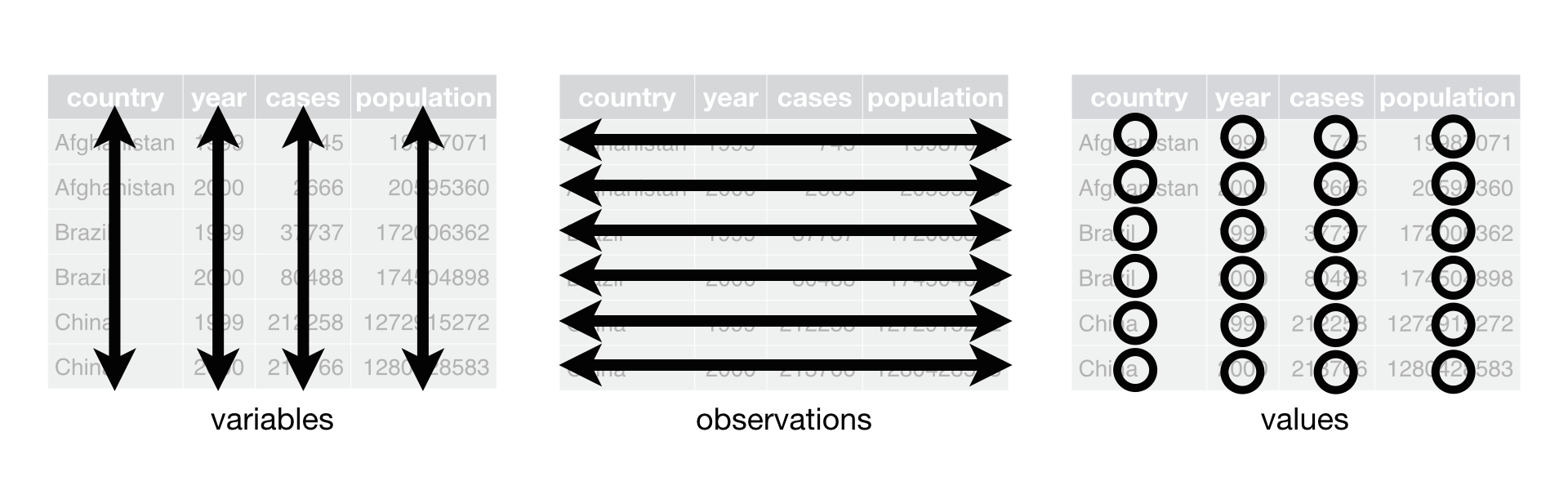
Source: Wickham & Grolemund (2023).
Wickham, H., & Grolemund, G. (2023). R for data science (2e). https://r4ds.hadley.nz/
Whenever data follow that consistent structure, we speak of tidy data. The underlying uniformity of tidy data facilitates learning and using data manipulation tools.
One difference between data frames and tibbles is that dataframes store the row names. For example, take the mtcars dataset which consists of 32 different cars and the names of the cars are not stored as rownames:
class(mtcars) # mtcars is a data frame[1] "data.frame"rownames(mtcars) [1] "Mazda RX4" "Mazda RX4 Wag" "Datsun 710"
[4] "Hornet 4 Drive" "Hornet Sportabout" "Valiant"
[7] "Duster 360" "Merc 240D" "Merc 230"
[10] "Merc 280" "Merc 280C" "Merc 450SE"
[13] "Merc 450SL" "Merc 450SLC" "Cadillac Fleetwood"
[16] "Lincoln Continental" "Chrysler Imperial" "Fiat 128"
[19] "Honda Civic" "Toyota Corolla" "Toyota Corona"
[22] "Dodge Challenger" "AMC Javelin" "Camaro Z28"
[25] "Pontiac Firebird" "Fiat X1-9" "Porsche 914-2"
[28] "Lotus Europa" "Ford Pantera L" "Ferrari Dino"
[31] "Maserati Bora" "Volvo 142E" To store mtcars as a tibble, we can use the as_tibble function:
tbl_mtcars <- as_tibble(mtcars)
class(tbl_mtcars) # check if it is a tibble now
[1] "tbl_df" "tbl" "data.frame"is_tibble(tbl_mtcars) # alternative check[1] TRUEhead(tbl_mtcars, 3)# A tibble: 3 × 11
mpg cyl disp hp drat wt qsec vs am gear carb
<dbl> <dbl> <dbl> <dbl> <dbl> <dbl> <dbl> <dbl> <dbl> <dbl> <dbl>
1 21 6 160 110 3.9 2.62 16.5 0 1 4 4
2 21 6 160 110 3.9 2.88 17.0 0 1 4 4
3 22.8 4 108 93 3.85 2.32 18.6 1 1 4 1When we look at the data, we’ve lost the names of the cars. To store the these, you need to first add a column to the dataframe containing the rownames and then you can generate the tibble:
tbl_mtcars <- mtcars |>
  rownames_to_column(var = "car") |>
  as_tibble()
class(tbl_mtcars)
[1] "tbl_df" "tbl" "data.frame"head(tbl_mtcars, 3)# A tibble: 3 × 12
car mpg cyl disp hp drat wt qsec vs am gear carb
<chr> <dbl> <dbl> <dbl> <dbl> <dbl> <dbl> <dbl> <dbl> <dbl> <dbl> <dbl>
1 Mazda RX4 21 6 160 110 3.9 2.62 16.5 0 1 4 4
2 Mazda RX4 W… 21 6 160 110 3.9 2.88 17.0 0 1 4 4
3 Datsun 710 22.8 4 108 93 3.85 2.32 18.6 1 1 4 17.2.3 Data types
In R, different data classes, or types of data exist:
- numeric: can be any real number
- character: strings and characters
- integer: any whole numbers
- factor: any categorical or qualitative variable with finite number of distinct outcomes
- logical: contain either
TRUEorFALSE - Date: special format that describes time
The following example should exemplify these types of data:
integer_var <- c(1, 2, 3, 4, 5)
numeric_var <- c(1.1, 2.2, NA, 4.4, 5.5)
character_var <- c("apple", "banana", "orange", "cherry", "grape")
factor_var <- factor(c("red", "yellow", "red", "blue", "green"))
logical_var <- c(TRUE, TRUE, TRUE, FALSE, TRUE)
date_var <- as.Date(c("2022-01-01", "2022-02-01", "2022-03-01", "2022-04-01", "2022-05-01"))

date_var[2] - date_var[5] # number of days in between these two dates
Time difference of -89 daysThere are some special data values used in R that needs further explanation:
NAstands for not available or missing and is used to represent missing or undefined values.Infstands for infinity and is used to represent mathematical infinity, such as the result of dividing a non-zero number by zero. Can be positive or negative.
NULLrepresents an empty or non-existent object. It is often used as a placeholder when a value or object is not yet available or when an object is intentionally removed.NaNstands for not a number and is used to represent an undefined or unrepresentable value, such as the result of taking the square root of a negative number. It can also occur as a result of certain arithmetic operations that are undefined. In contrast toNAit can only exist in numerical data.
7.3 Operators
An overview of the most important operators of R is proided in Appendix B.
7.3.1 Algebraic operators
R can perform any kind of arithmetic calculation using the operators listed in Table 7.1.
| Operation | Operator | Example input | Example output |
|---|---|---|---|
| addition | + |
10+2 | 12 |
| subtraction | - |
9-3 | 6 |
| multiplication | * |
5*5 | 25 |
| division | / |
10/3 | 3 |
| power | ^ |
5^2 | 25 |
7.3.2 The pipe operator: |>
The pipe operator, %>%, comes from the magrittr package, which is also part of the tidyverse package. The pipe operator, |>, has been part of base R since version 4.1.0. For most cases, these two operators are identical. The pipe operator is designed to help you write code in a way that is easier to read and understand. As R is a functional language, code often contains a lot of parentheses, ( and ). Nesting these parentheses together can be complex and make your R code hard to read and understand, which is where |> comes to the rescue! It allows you to use the output of a function as the input of the next function.
Tip 7.1: Set the native pipe in RStudio
With the keyboard shortcut Ctrl+Shift+M, RStudio inserts %>%. To change that behavior, simply check the box labeled “Use native pipe operator, |>” in the Global Options, see: Tools > Global Options > Code > Editing.
Consider the following example of code to explain the usage of the pipe operator:
# create some data `x`
x <- c(1, 1.002, 1.004, .99, .99)
# take the logarithm of `x`,
log_x <- log(x)
# compute the lagged and iterated differences (see `diff()`)
growth_rate_x <- diff(log_x)
growth_rate_x
[1] 0.001998003 0.001994019 -0.014042357 0.000000000# round the result (4 digit)
growth_rate_x_round <- round(growth_rate_x, 4)
growth_rate_x_round[1] 0.002 0.002 -0.014 0.000That is rather long and we actually don’t need objects log_x, growth_rate_x, and growth_rate_x_round. Well, then let us write that in a nested function:
round(diff(log(x)), 4)[1] 0.002 0.002 -0.014 0.000This is short but hard to read and understand. The solution is the “pipe”:
# load one of these packages: `magrittr` or `tidyverse`
library(tidyverse)

# Perform the same computations on `x` as above
x |>
  log() |>
  diff() |>
  round(4)
[1] 0.002 0.002 -0.014 0.000You can read the |> with “and then” because it takes the results of some function “and then” does something with that in the next. For example, reading out loud the following code would sound something like this:
- I take the mtcars data, and then
- I consider only cars with more than 4 cylinders, and then
- I group the cars by the number of cylinders the cars have, and then
- I summarize the data and show the means of miles per gallon (mpg) and horse powers (hp) by groups of cars that distinguish by their number of cylinders.
mtcars |>
  filter(cyl > 4) |>
  group_by(cyl) |>
  summarise_at(c("mpg", "hp"), mean)
# A tibble: 2 × 3
cyl mpg hp
<dbl> <dbl> <dbl>
1 6 19.7 122.
2 8 15.1 209.7.3.3 The %in% operator
%in% is used to subset a vector by comparison. Here’s an example:
x <- c(1, 3, 5, 7)
y <- c(2, 4, 6, 8)
z <- c(1, 2, 3)

x %in% y
[1] FALSE FALSE FALSE FALSEx %in% z[1] TRUE TRUE FALSE FALSEz %in% x[1] TRUE FALSE TRUEThe %in% operator can be used in combination with other functions like subset() and filter().
7.3.4 Extract operators
The extract operators are used to retrieve data from objects in R. The operator may take four forms, including [], [[]], and $.
[] allows to extract content from vector, lists, or data frames. For example,
a <- mtcars[3, ]
b <- mtcars["Datsun 710", ]
identical(a, b)
[1] TRUEa mpg cyl disp hp drat wt qsec vs am gear carb
Datsun 710 22.8 4 108 93 3.85 2.32 18.61 1 1 4 1extracts the third observation of the mtcars dataset, and
c <- mtcars[, "cyl"]
d <- mtcars[, 2]
identical(x, y)
[1] FALSEc [1] 6 6 4 6 8 6 8 4 4 6 6 8 8 8 8 8 8 4 4 4 4 8 8 8 8 4 4 4 8 6 8 4extracts the variable/vector cyl.
The operators, [[]] and $ extract a single item from an object. It is used to refer to an element in a list or a column in a data frame. For example,
e <- mtcars$cyl
f <- mtcars[["cyl"]]
identical(e, f)
[1] TRUEe [1] 6 6 4 6 8 6 8 4 4 6 6 8 8 8 8 8 8 4 4 4 4 8 8 8 8 4 4 4 8 6 8 4will return the values of the variable cyl from the data frame mtcars. Thus, x$y is actually just a short form for x[[“y”]].
7.3.5 Logical operators
The extract operators can be combined with the logical operators (more precisely, I should call these binary relational operators) that are shown in Table 7.2.
| operation | operator | example input | answer |
|---|---|---|---|
| less than | < |
2 < 3 |
TRUE |
| less than or equal to | <= |
2 <= 2 |
TRUE |
| greater than | > |
2 > 3 |
FALSE |
| greater than or equal to | >= |
2 >= 2 |
TRUE |
| equal to | == |
2 == 3 |
FALSE |
| not equal to | != |
2 != 3 |
TRUE |
| not | ! |
!(1==1) |
FALSE |
| or | \(\vert\) | (1==1) \(\vert\) (2==3) |
TRUE |
| and | & |
(1==1) & (2==3) |
FALSE |
Here are some examples: Select rows where the number of cylinders is greater than or equal to 6:
mtcars[mtcars$cyl >= 6, ] mpg cyl disp hp drat wt qsec vs am gear carb
Mazda RX4 21.0 6 160.0 110 3.90 2.620 16.46 0 1 4 4
Mazda RX4 Wag 21.0 6 160.0 110 3.90 2.875 17.02 0 1 4 4
Hornet 4 Drive 21.4 6 258.0 110 3.08 3.215 19.44 1 0 3 1
Hornet Sportabout 18.7 8 360.0 175 3.15 3.440 17.02 0 0 3 2
Valiant 18.1 6 225.0 105 2.76 3.460 20.22 1 0 3 1
Duster 360 14.3 8 360.0 245 3.21 3.570 15.84 0 0 3 4
Merc 280 19.2 6 167.6 123 3.92 3.440 18.30 1 0 4 4
Merc 280C 17.8 6 167.6 123 3.92 3.440 18.90 1 0 4 4
Merc 450SE 16.4 8 275.8 180 3.07 4.070 17.40 0 0 3 3
Merc 450SL 17.3 8 275.8 180 3.07 3.730 17.60 0 0 3 3
Merc 450SLC 15.2 8 275.8 180 3.07 3.780 18.00 0 0 3 3
Cadillac Fleetwood 10.4 8 472.0 205 2.93 5.250 17.98 0 0 3 4
Lincoln Continental 10.4 8 460.0 215 3.00 5.424 17.82 0 0 3 4
Chrysler Imperial 14.7 8 440.0 230 3.23 5.345 17.42 0 0 3 4
Dodge Challenger 15.5 8 318.0 150 2.76 3.520 16.87 0 0 3 2
AMC Javelin 15.2 8 304.0 150 3.15 3.435 17.30 0 0 3 2
Camaro Z28 13.3 8 350.0 245 3.73 3.840 15.41 0 0 3 4
Pontiac Firebird 19.2 8 400.0 175 3.08 3.845 17.05 0 0 3 2
Ford Pantera L 15.8 8 351.0 264 4.22 3.170 14.50 0 1 5 4
Ferrari Dino 19.7 6 145.0 175 3.62 2.770 15.50 0 1 5 6
Maserati Bora 15.0 8 301.0 335 3.54 3.570 14.60 0 1 5 8Select rows where the number of cylinders is either 4 or 6:
mtcars[mtcars$cyl == 4 | mtcars$cyl == 6, ] mpg cyl disp hp drat wt qsec vs am gear carb
Mazda RX4 21.0 6 160.0 110 3.90 2.620 16.46 0 1 4 4
Mazda RX4 Wag 21.0 6 160.0 110 3.90 2.875 17.02 0 1 4 4
Datsun 710 22.8 4 108.0 93 3.85 2.320 18.61 1 1 4 1
Hornet 4 Drive 21.4 6 258.0 110 3.08 3.215 19.44 1 0 3 1
Valiant 18.1 6 225.0 105 2.76 3.460 20.22 1 0 3 1
Merc 240D 24.4 4 146.7 62 3.69 3.190 20.00 1 0 4 2
Merc 230 22.8 4 140.8 95 3.92 3.150 22.90 1 0 4 2
Merc 280 19.2 6 167.6 123 3.92 3.440 18.30 1 0 4 4
Merc 280C 17.8 6 167.6 123 3.92 3.440 18.90 1 0 4 4
Fiat 128 32.4 4 78.7 66 4.08 2.200 19.47 1 1 4 1
Honda Civic 30.4 4 75.7 52 4.93 1.615 18.52 1 1 4 2
Toyota Corolla 33.9 4 71.1 65 4.22 1.835 19.90 1 1 4 1
Toyota Corona 21.5 4 120.1 97 3.70 2.465 20.01 1 0 3 1
Fiat X1-9 27.3 4 79.0 66 4.08 1.935 18.90 1 1 4 1
Porsche 914-2 26.0 4 120.3 91 4.43 2.140 16.70 0 1 5 2
Lotus Europa 30.4 4 95.1 113 3.77 1.513 16.90 1 1 5 2
Ferrari Dino 19.7 6 145.0 175 3.62 2.770 15.50 0 1 5 6
Volvo 142E 21.4 4 121.0 109 4.11 2.780 18.60 1 1 4 2Select rows where the number of cylinders is 4 and the mpg is greater than 22:
mtcars[mtcars$cyl == 4 & mtcars$mpg > 22, ] mpg cyl disp hp drat wt qsec vs am gear carb
Datsun 710 22.8 4 108.0 93 3.85 2.320 18.61 1 1 4 1
Merc 240D 24.4 4 146.7 62 3.69 3.190 20.00 1 0 4 2
Merc 230 22.8 4 140.8 95 3.92 3.150 22.90 1 0 4 2
Fiat 128 32.4 4 78.7 66 4.08 2.200 19.47 1 1 4 1
Honda Civic 30.4 4 75.7 52 4.93 1.615 18.52 1 1 4 2
Toyota Corolla 33.9 4 71.1 65 4.22 1.835 19.90 1 1 4 1
Fiat X1-9 27.3 4 79.0 66 4.08 1.935 18.90 1 1 4 1
Porsche 914-2 26.0 4 120.3 91 4.43 2.140 16.70 0 1 5 2
Lotus Europa 30.4 4 95.1 113 3.77 1.513 16.90 1 1 5 2Select rows where the weight is less than 3.5 or the number of gears is greater than 4:
mtcars[mtcars$wt < 3.5 | mtcars$gear > 4, ] mpg cyl disp hp drat wt qsec vs am gear carb
Mazda RX4 21.0 6 160.0 110 3.90 2.620 16.46 0 1 4 4
Mazda RX4 Wag 21.0 6 160.0 110 3.90 2.875 17.02 0 1 4 4
Datsun 710 22.8 4 108.0 93 3.85 2.320 18.61 1 1 4 1
Hornet 4 Drive 21.4 6 258.0 110 3.08 3.215 19.44 1 0 3 1
Hornet Sportabout 18.7 8 360.0 175 3.15 3.440 17.02 0 0 3 2
Valiant 18.1 6 225.0 105 2.76 3.460 20.22 1 0 3 1
Merc 240D 24.4 4 146.7 62 3.69 3.190 20.00 1 0 4 2
Merc 230 22.8 4 140.8 95 3.92 3.150 22.90 1 0 4 2
Merc 280 19.2 6 167.6 123 3.92 3.440 18.30 1 0 4 4
Merc 280C 17.8 6 167.6 123 3.92 3.440 18.90 1 0 4 4
Fiat 128 32.4 4 78.7 66 4.08 2.200 19.47 1 1 4 1
Honda Civic 30.4 4 75.7 52 4.93 1.615 18.52 1 1 4 2
Toyota Corolla 33.9 4 71.1 65 4.22 1.835 19.90 1 1 4 1
Toyota Corona 21.5 4 120.1 97 3.70 2.465 20.01 1 0 3 1
AMC Javelin 15.2 8 304.0 150 3.15 3.435 17.30 0 0 3 2
Fiat X1-9 27.3 4 79.0 66 4.08 1.935 18.90 1 1 4 1
Porsche 914-2 26.0 4 120.3 91 4.43 2.140 16.70 0 1 5 2
Lotus Europa 30.4 4 95.1 113 3.77 1.513 16.90 1 1 5 2
Ford Pantera L 15.8 8 351.0 264 4.22 3.170 14.50 0 1 5 4
Ferrari Dino 19.7 6 145.0 175 3.62 2.770 15.50 0 1 5 6
Maserati Bora 15.0 8 301.0 335 3.54 3.570 14.60 0 1 5 8
Volvo 142E 21.4 4 121.0 109 4.11 2.780 18.60 1 1 4 2Select rows where either mpg is greater than 25 or carb is less than 2, and the number of cylinders is either 4 or 8.
mtcars[(mtcars$mpg > 25 | mtcars$carb < 2) & mtcars$cyl %in% c(4, 8), ] mpg cyl disp hp drat wt qsec vs am gear carb
Datsun 710 22.8 4 108.0 93 3.85 2.320 18.61 1 1 4 1
Fiat 128 32.4 4 78.7 66 4.08 2.200 19.47 1 1 4 1
Honda Civic 30.4 4 75.7 52 4.93 1.615 18.52 1 1 4 2
Toyota Corolla 33.9 4 71.1 65 4.22 1.835 19.90 1 1 4 1
Toyota Corona 21.5 4 120.1 97 3.70 2.465 20.01 1 0 3 1
Fiat X1-9 27.3 4 79.0 66 4.08 1.935 18.90 1 1 4 1
Porsche 914-2 26.0 4 120.3 91 4.43 2.140 16.70 0 1 5 2
Lotus Europa 30.4 4 95.1 113 3.77 1.513 16.90 1 1 5 27.4 Data manipulation
7.4.1 dplyr: A human readable grammar of data manipulation
dplyr package
The dplyr package is part of tidyverse and makes data manipulation easy as it works well with the pipe operator |>. The most important function are the following:
- Reorder the rows with
arrange(). - Pick observations by their values with
filter(). - Pick variables by their names with
select(). - Create new variables with functions of existing variables with
mutate(). - Collapse many values down to a single summary with
summarise(). - Rename variables with
rename(). - Change the position of variables with
relocate().
These functions can be used in conjunction with group_by() and/or rowwise(), which changes the scope of each function from operating on the entire dataset to operating on it group-by-group or by rows. Moreover, you can check for conditions and take action with, for example, if_else() and case_when().
All functions work similarly:
- The first argument is a data frame.
- The subsequent arguments describe what to do with the data frame.
- The result is a new data frame.
Here are some examples that may help to understand these functions:
library(tidyverse)

# load mtcars dataset
data(mtcars)

# filter only cars with four gears
mtcars_gear_4 <- mtcars |>
  filter(gear == 4)

# arrange rows by mpg in descending order
mtcars_gear_4 |>
  arrange(desc(mpg))
mpg cyl disp hp drat wt qsec vs am gear carb
Toyota Corolla 33.9 4 71.1 65 4.22 1.835 19.90 1 1 4 1
Fiat 128 32.4 4 78.7 66 4.08 2.200 19.47 1 1 4 1
Honda Civic 30.4 4 75.7 52 4.93 1.615 18.52 1 1 4 2
Fiat X1-9 27.3 4 79.0 66 4.08 1.935 18.90 1 1 4 1
Merc 240D 24.4 4 146.7 62 3.69 3.190 20.00 1 0 4 2
Datsun 710 22.8 4 108.0 93 3.85 2.320 18.61 1 1 4 1
Merc 230 22.8 4 140.8 95 3.92 3.150 22.90 1 0 4 2
Volvo 142E 21.4 4 121.0 109 4.11 2.780 18.60 1 1 4 2
Mazda RX4 21.0 6 160.0 110 3.90 2.620 16.46 0 1 4 4
Mazda RX4 Wag 21.0 6 160.0 110 3.90 2.875 17.02 0 1 4 4
Merc 280 19.2 6 167.6 123 3.92 3.440 18.30 1 0 4 4
Merc 280C 17.8 6 167.6 123 3.92 3.440 18.90 1 0 4 4# Change the order of the variables
glimpse(mtcars_gear_4)Rows: 12
Columns: 11
$ mpg <dbl> 21.0, 21.0, 22.8, 24.4, 22.8, 19.2, 17.8, 32.4, 30.4, 33.9, 27.3,…
$ cyl <dbl> 6, 6, 4, 4, 4, 6, 6, 4, 4, 4, 4, 4
$ disp <dbl> 160.0, 160.0, 108.0, 146.7, 140.8, 167.6, 167.6, 78.7, 75.7, 71.1…
$ hp <dbl> 110, 110, 93, 62, 95, 123, 123, 66, 52, 65, 66, 109
$ drat <dbl> 3.90, 3.90, 3.85, 3.69, 3.92, 3.92, 3.92, 4.08, 4.93, 4.22, 4.08,…
$ wt <dbl> 2.620, 2.875, 2.320, 3.190, 3.150, 3.440, 3.440, 2.200, 1.615, 1.…
$ qsec <dbl> 16.46, 17.02, 18.61, 20.00, 22.90, 18.30, 18.90, 19.47, 18.52, 19…
$ vs <dbl> 0, 0, 1, 1, 1, 1, 1, 1, 1, 1, 1, 1
$ am <dbl> 1, 1, 1, 0, 0, 0, 0, 1, 1, 1, 1, 1
$ gear <dbl> 4, 4, 4, 4, 4, 4, 4, 4, 4, 4, 4, 4
$ carb <dbl> 4, 4, 1, 2, 2, 4, 4, 1, 2, 1, 1, 2mtcars_gear_4 |>
relocate(cyl, disp, carb) |>
glimpse()Rows: 12
Columns: 11
$ cyl <dbl> 6, 6, 4, 4, 4, 6, 6, 4, 4, 4, 4, 4
$ disp <dbl> 160.0, 160.0, 108.0, 146.7, 140.8, 167.6, 167.6, 78.7, 75.7, 71.1…
$ carb <dbl> 4, 4, 1, 2, 2, 4, 4, 1, 2, 1, 1, 2
$ mpg <dbl> 21.0, 21.0, 22.8, 24.4, 22.8, 19.2, 17.8, 32.4, 30.4, 33.9, 27.3,…
$ hp <dbl> 110, 110, 93, 62, 95, 123, 123, 66, 52, 65, 66, 109
$ drat <dbl> 3.90, 3.90, 3.85, 3.69, 3.92, 3.92, 3.92, 4.08, 4.93, 4.22, 4.08,…
$ wt <dbl> 2.620, 2.875, 2.320, 3.190, 3.150, 3.440, 3.440, 2.200, 1.615, 1.…
$ qsec <dbl> 16.46, 17.02, 18.61, 20.00, 22.90, 18.30, 18.90, 19.47, 18.52, 19…
$ vs <dbl> 0, 0, 1, 1, 1, 1, 1, 1, 1, 1, 1, 1
$ am <dbl> 1, 1, 1, 0, 0, 0, 0, 1, 1, 1, 1, 1
$ gear <dbl> 4, 4, 4, 4, 4, 4, 4, 4, 4, 4, 4, 4mtcars_gear_4 |>
relocate(sort(names(mtcars_gear_4))) |>
glimpse()Rows: 12
Columns: 11
$ am <dbl> 1, 1, 1, 0, 0, 0, 0, 1, 1, 1, 1, 1
$ carb <dbl> 4, 4, 1, 2, 2, 4, 4, 1, 2, 1, 1, 2
$ cyl <dbl> 6, 6, 4, 4, 4, 6, 6, 4, 4, 4, 4, 4
$ disp <dbl> 160.0, 160.0, 108.0, 146.7, 140.8, 167.6, 167.6, 78.7, 75.7, 71.1…
$ drat <dbl> 3.90, 3.90, 3.85, 3.69, 3.92, 3.92, 3.92, 4.08, 4.93, 4.22, 4.08,…
$ gear <dbl> 4, 4, 4, 4, 4, 4, 4, 4, 4, 4, 4, 4
$ hp <dbl> 110, 110, 93, 62, 95, 123, 123, 66, 52, 65, 66, 109
$ mpg <dbl> 21.0, 21.0, 22.8, 24.4, 22.8, 19.2, 17.8, 32.4, 30.4, 33.9, 27.3,…
$ qsec <dbl> 16.46, 17.02, 18.61, 20.00, 22.90, 18.30, 18.90, 19.47, 18.52, 19…
$ vs <dbl> 0, 0, 1, 1, 1, 1, 1, 1, 1, 1, 1, 1
$ wt <dbl> 2.620, 2.875, 2.320, 3.190, 3.150, 3.440, 3.440, 2.200, 1.615, 1.…# filter rows where cyl = 4
mtcars_gear_4 |>
filter(cyl == 4) mpg cyl disp hp drat wt qsec vs am gear carb
Datsun 710 22.8 4 108.0 93 3.85 2.320 18.61 1 1 4 1
Merc 240D 24.4 4 146.7 62 3.69 3.190 20.00 1 0 4 2
Merc 230 22.8 4 140.8 95 3.92 3.150 22.90 1 0 4 2
Fiat 128 32.4 4 78.7 66 4.08 2.200 19.47 1 1 4 1
Honda Civic 30.4 4 75.7 52 4.93 1.615 18.52 1 1 4 2
Toyota Corolla 33.9 4 71.1 65 4.22 1.835 19.90 1 1 4 1
Fiat X1-9 27.3 4 79.0 66 4.08 1.935 18.90 1 1 4 1
Volvo 142E 21.4 4 121.0 109 4.11 2.780 18.60 1 1 4 2# select columns mpg, cyl, and hp
mtcars_gear_4 |>
select(mpg, cyl, hp) |>
head() mpg cyl hp
Mazda RX4 21.0 6 110
Mazda RX4 Wag 21.0 6 110
Datsun 710 22.8 4 93
Merc 240D 24.4 4 62
Merc 230 22.8 4 95
Merc 280 19.2 6 123# select columns all variables except wt and hp
mtcars_gear_4 |>
select(-wt, -hp) |>
head() mpg cyl disp drat qsec vs am gear carb
Mazda RX4 21.0 6 160.0 3.90 16.46 0 1 4 4
Mazda RX4 Wag 21.0 6 160.0 3.90 17.02 0 1 4 4
Datsun 710 22.8 4 108.0 3.85 18.61 1 1 4 1
Merc 240D 24.4 4 146.7 3.69 20.00 1 0 4 2
Merc 230 22.8 4 140.8 3.92 22.90 1 0 4 2
Merc 280 19.2 6 167.6 3.92 18.30 1 0 4 4# select only variables starting with `c`
mtcars_gear_4 |>
select(starts_with("c")) cyl carb
Mazda RX4 6 4
Mazda RX4 Wag 6 4
Datsun 710 4 1
Merc 240D 4 2
Merc 230 4 2
Merc 280 6 4
Merc 280C 6 4
Fiat 128 4 1
Honda Civic 4 2
Toyota Corolla 4 1
Fiat X1-9 4 1
Volvo 142E 4 2# summarize avg mpg by number of cylinders
mtcars_gear_4 |>
group_by(cyl) |>
summarize(avg_mpg = mean(mpg))# A tibble: 2 × 2
cyl avg_mpg
<dbl> <dbl>
1 4 26.9
2 6 19.8# create new column wt_kg, which is wt in kg
mtcars_gear_4 |>
select(wt) |>
mutate(wt_kg = wt / 2.205) |>
head() wt wt_kg
Mazda RX4 2.620 1.188209
Mazda RX4 Wag 2.875 1.303855
Datsun 710 2.320 1.052154
Merc 240D 3.190 1.446712
Merc 230 3.150 1.428571
Merc 280 3.440 1.560091# Create a new variable by calculating hp divided by wt
mtcars_new <- mtcars |>
select(wt, hp) |>
mutate(hp_per_t = hp / wt) |>
head()
# Print the first few rows of the updated dataset
head(mtcars_new) wt hp hp_per_t
Mazda RX4 2.620 110 41.98473
Mazda RX4 Wag 2.875 110 38.26087
Datsun 710 2.320 93 40.08621
Hornet 4 Drive 3.215 110 34.21462
Hornet Sportabout 3.440 175 50.87209
Valiant 3.460 105 30.34682# Rename hp to horsepower
mtcars_gear_4 |>
rename(horsepower = hp) |>
glimpse()Rows: 12
Columns: 11
$ mpg <dbl> 21.0, 21.0, 22.8, 24.4, 22.8, 19.2, 17.8, 32.4, 30.4, 33.9,…
$ cyl <dbl> 6, 6, 4, 4, 4, 6, 6, 4, 4, 4, 4, 4
$ disp <dbl> 160.0, 160.0, 108.0, 146.7, 140.8, 167.6, 167.6, 78.7, 75.7…
$ horsepower <dbl> 110, 110, 93, 62, 95, 123, 123, 66, 52, 65, 66, 109
$ drat <dbl> 3.90, 3.90, 3.85, 3.69, 3.92, 3.92, 3.92, 4.08, 4.93, 4.22,…
$ wt <dbl> 2.620, 2.875, 2.320, 3.190, 3.150, 3.440, 3.440, 2.200, 1.6…
$ qsec <dbl> 16.46, 17.02, 18.61, 20.00, 22.90, 18.30, 18.90, 19.47, 18.…
$ vs <dbl> 0, 0, 1, 1, 1, 1, 1, 1, 1, 1, 1, 1
$ am <dbl> 1, 1, 1, 0, 0, 0, 0, 1, 1, 1, 1, 1
$ gear <dbl> 4, 4, 4, 4, 4, 4, 4, 4, 4, 4, 4, 4
$ carb <dbl> 4, 4, 1, 2, 2, 4, 4, 1, 2, 1, 1, 27.4.2 If statements
In many cases, it’s necessary to execute certain code only when a particular condition is met. To achieve this, there are several conditional statements that can be used in code. These include:
- The
ifstatement: This is used to execute a block of code if a specified condition is true. - The
elsestatement: This is used to execute a block of code if the same condition is false. - The
elseif statement: This is used to specify a new condition to test if the first condition is false. - The
if_else()function: This is used to check a condition for every element of a vector.
The following examples should exemplify how these statements work:
# Example of if statement
if (mean(mtcars$mpg) > 20) {
  print("The average miles per gallon is greater than 20.")
}
[1] "The average miles per gallon is greater than 20."# Example of if-else statement
if (mean(mtcars$mpg) > 20) {
print("The average miles per gallon is greater than 20.")
} else {
print("The average miles per gallon is less than or equal to 20.")
}[1] "The average miles per gallon is greater than 20."# Example of if-else if statement
if (mean(mtcars$mpg) > 25) {
print("The average miles per gallon is greater than 25.")
} else if (mean(mtcars$mpg) > 20) {
print("The average miles per gallon is between 20 and 25.")
} else {
print("The average miles per gallon is less than or equal to 20.")
}[1] "The average miles per gallon is between 20 and 25."# Example of if_else function
mtcars_2 <- mtcars
mtcars_2$mpg_category <- if_else(mtcars_2$mpg > 20, "High", "Low")When you have a fixed number of cases and don’t want to use a long chain of if-else statements, you can use case_when();
mtcars_cyl <- mtcars |>
  mutate(cyl_category = case_when(
    cyl == 4 ~ "four",
    cyl == 6 ~ "six",
    cyl == 8 ~ "eight"
  ))
The mutate() function is used to add the new variable, and case_when() is used to assign the values “four”, “six”, or “eight” to the new variable based on the number of cylinders in each car. Both functions are part of the dplyr package (see chapter Section 7.4.1).
7.4.3 Examining and cleaning data with the janitor package
The janitor package follows the principles of the tidyverse and works well with the pipe operator |>. The janitor functions has many usefull functions for the initial data exploration and cleaning that are essential when you load any new data set.
First, make sure the janitor package is installed and loaded:
7.4.3.1 Clean data.frame names with clean_names()
I call this function frequently when I read in new data. It handles problematic variable names, especially those that are so well-preserved by readxl::read_excel() and readr::read_csv(). For example, it does the following:
- Parses letter cases and separators to a consistent format.
- Handles special characters and spaces, including transliterating characters like
œtooe. - Appends numbers to duplicated names
- Converts “%” to “percent” and “#” to “number” to retain meaning
- Spacing (or lack thereof) around numbers is preserved
To exemplify what it does, let’s create some data with akward names and then clean them:
df_test <- as.data.frame(matrix(ncol = 6))
names(df_test) <- c(
  "firstName", "ábc@!*", "% successful (2009)",
  "REPEAT VALUE", "REPEAT VALUE", ""
)
df_cln <- df_test |>
  clean_names()
names(df_test)
[1] "firstName" "ábc@!*" "% successful (2009)"
[4] "REPEAT VALUE" "REPEAT VALUE" "" names(df_cln)[1] "first_name" "abc"
[3] "percent_successful_2009" "repeat_value"
[5] "repeat_value_2" "x" 7.4.3.2 Find duplicated values for specific combinations of variables with get_dupes()
get_dupes allows you to check for the indentifying variable. In other words, it shows you duplicates for specific combinations of variables.
For example, consider the following tibble:
df_panel <- tibble(
  country = c(rep("a", 3), rep("b", 3), rep("c", 3)),
  year = rep(1:3, 3),
  GDP = c(1000, 2000, 3000, 4000, 5000, 6000, 7000, 8000, 9000)
)
df_panel
# A tibble: 9 × 3
country year GDP
<chr> <int> <dbl>
1 a 1 1000
2 a 2 2000
3 a 3 3000
4 b 1 4000
5 b 2 5000
6 b 3 6000
7 c 1 7000
8 c 2 8000
9 c 3 9000with
get_dupes(df_panel, country, year)No duplicate combinations found of: country, year# A tibble: 0 × 4
# ℹ 4 variables: country <chr>, year <int>, dupe_count <int>, GDP <dbl>we see that this is a panel dataset identified by a combination of country and year. Now let us introduce a duplicate and check again:
new_obs <- tibble(country = "b", year = 2, GDP = 5000)
df_panel_dup <- bind_rows(df_panel, new_obs)
get_dupes(df_panel_dup, country, year)
# A tibble: 2 × 4
country year dupe_count GDP
<chr> <dbl> <int> <dbl>
1 b 2 2 5000
2 b 2 2 5000
Tip 7.2: The
plm package
Speaking of panel datasets, it’s worth mentioning the plm package, which is excellent for managing such data. For example, you can use is.pbalanced to verify whether a panel is balanced, meaning it has the same years for all countries.
pacman::p_load(plm)
is.pbalanced(df_panel)
[1] TRUEIf your panel is unbalanced, you can use make.pbalanced to rectify it:
df_unbal <- df_panel |>
  filter(row_number() != 7)
df_unbal
# A tibble: 8 × 3
country year GDP
<chr> <int> <dbl>
1 a 1 1000
2 a 2 2000
3 a 3 3000
4 b 1 4000
5 b 2 5000
6 b 3 6000
7 c 2 8000
8 c 3 9000is.pbalanced(df_unbal)[1] FALSEdf_unbal_balanced <- make.pbalanced(df_unbal)
df_unbal_balanced country year GDP
1 a 1 1000
2 a 2 2000
3 a 3 3000
4 b 1 4000
5 b 2 5000
6 b 3 6000
7 c 1 NA
8 c 2 8000
9 c 3 90007.4.3.3 remove_empty() rows and columns
For cleaning Excel files that contain empty rows and columns after being read into R, remove_empty can be very helpful:
q <- data.frame(
  v1 = c(1, NA, 3),
  v2 = c(NA, NA, NA),
  v3 = c("a", NA, "b")
)
q |>
  remove_empty(c("rows", "cols"))
v1 v3
1 1 a
3 3 b7.4.3.4 remove_constant() columns
Removes variables from data that contain only a single constant value (with an na.rm option to control whether NAs should be considered as different values from the constant).
a <- data.frame(good = 1:3, boring = "the same")
a
good boring
1 1 the same
2 2 the same
3 3 the samea |>
remove_constant() good
1 1
2 2
3 37.4.4 tabyl() - a better version of table()
tabyl() is a tidyverse-oriented replacement for table(). It counts combinations of one, two, or three variables, and then can be formatted with a suite of adorn_* functions to look just how you want. For example:
mtcars |>
  tabyl(gear, cyl) |>
  adorn_totals("col") |>
  adorn_percentages("row") |>
  adorn_pct_formatting(digits = 2) |>
  adorn_ns() |>
  adorn_title()
cyl
gear 4 6 8 Total
3 6.67% (1) 13.33% (2) 80.00% (12) 100.00% (15)
4 66.67% (8) 33.33% (4) 0.00% (0) 100.00% (12)
5 40.00% (2) 20.00% (1) 40.00% (2) 100.00% (5)Learn more in the tabyls vignette.
7.5 User-defined functions and conflicts
One of the great strengths of R is the user’s ability to add functions. Sometimes there is a small task (or series of tasks) you need done and you find yourself having to repeat it multiple times. In these types of situations it can be helpful to create your own custom function. The structure of a function is given below:
name_of_function <- function(argument1, argument2) {
    statements or code that does something
    return(something)
}
First you give your function a name. Then you assign value to it, where the value is the function. When defining the function you will want to provide the list of arguments required (inputs and/or options to modify behavior of the function), and wrapped between curly brackets place the tasks that are being executed on/using those arguments. The argument(s) can be any type of object (like a scalar, a matrix, a dataframe, a vector, a logical, etc), and it’s not necessary to define what it is in any way. Finally, you can return the value of the object from the function, meaning pass the value of it into the global environment. The important idea behind functions is that objects that are created within the function are local to the environment of the function – they don’t exist outside of the function. Note, a function doesn’t require any arguments.
Let’s try creating a simple example function. This function will take in a numeric value as input, and return the squared value.
square_it <- function(x) {
   square <- x * x
   return(square)
}
Now, we can use the function as we would any other function. We type out the name of the function, and inside the parentheses we provide a numeric value x:
square_it(5)[1] 25Let us get back to script with sales and try to calculate the monthly growth rates of revenue using a self-written function.
The formula of a growth rate is clear:
\[ g=\left(\frac{y_t-y_{t-1}}{y_{t-1}}\right)\cdot 100=\left(\frac{y_t}{y_{t-1}}-1\right)\cdot 100 \]
So the challenge is to divide the value of revenue with the value of the previous period, a.k.a. the lagged value. Let us assume that the function lag() can give you exactly that value of a vector. Lets try it out:
lag(revenue) [1] 0 700 1400 350 175 28 56 0 0 0 0 0
attr(,"tsp")
[1] 0 11 1(revenue/lag(revenue)-1)*100 [1] NaN 0 0 0 0 0 0 NaN NaN NaN NaN NaN
attr(,"tsp")
[1] 0 11 1Unfortunately, this does not work out. The lag() function does not work as we think it should. Well, the reason is simply that we are using the wrong function. The current lag() function is part of the stats package which is part of the package stats which is part of R base and is loaded automatically. The lag() function we aim to use stems from the dplyr package which we must install and load to be able to use it. So let’s do it:
# check if the package is installed
find.package("dplyr")
[1] "/usr/local/lib/R/site-library/dplyr"# I already installed the package so I can just load it
# install.packages("dplyr")
library("dplyr")
Attaching package: 'dplyr'The following objects are masked from 'package:plm':
between, lag, leadThe following objects are masked from 'package:stats':
filter, lagThe following objects are masked from 'package:base':
intersect, setdiff, setequal, unionThis message informs us that among other functions the lag() function is masked. That means that now the function of the newly loaded package is active. This is one example of why I highly recommend to unload all packages at the beginning of a script and then to use p_load to install and load the packages that should be used in the upcoming script:
pacman::p_unload(all)
pacman::p_load(dplyr)
So, let’s try again:
lag(revenue) [1] NA 0 700 1400 350 175 28 56 0 0 0 0(revenue/lag(revenue)-1)*100 [1] NA Inf 100 -75 -50 -84 100 -100 NaN NaN NaN NaNThat looks good now. And here is a way to calculate growth rates with a self-written function:
growth_rate <- function(x) {
  (x / lag(x) - 1) * 100
}
growth_rate(revenue)
[1] NA Inf 100 -75 -50 -84 100 -100 NaN NaN NaN NaNsales_gr_rate <- growth_rate(revenue)
sales_gr_rate [1] NA Inf 100 -75 -50 -84 100 -100 NaN NaN NaN NaNIn R, all functions are written by users, and it is not uncommon for two people to name their functions identically. In such cases, we must resolve the conflict by choosing which function to use. To use the lag function from the stats package, you can use the double colon operator :: like this stats::lag().
7.6 Example: How to explore a dataset
# Creating dataframe
df <- tibble(
  integer_var, numeric_var, character_var, factor_var, logical_var, date_var,
)

# Overview of the data
head(df)
# A tibble: 5 × 6
integer_var numeric_var character_var factor_var logical_var date_var
<dbl> <dbl> <chr> <fct> <lgl> <date>
1 1 1.1 apple red TRUE 2022-01-01
2 2 2.2 banana yellow TRUE 2022-02-01
3 3 NA orange red TRUE 2022-03-01
4 4 4.4 cherry blue FALSE 2022-04-01
5 5 5.5 grape green TRUE 2022-05-01summary(df) integer_var numeric_var character_var factor_var logical_var
Min. :1 Min. :1.100 Length:5 blue :1 Mode :logical
1st Qu.:2 1st Qu.:1.925 Class :character green :1 FALSE:1
Median :3 Median :3.300 Mode :character red :2 TRUE :4
Mean :3 Mean :3.300 yellow:1
3rd Qu.:4 3rd Qu.:4.675
Max. :5 Max. :5.500
NA's :1
date_var
Min. :2022-01-01
1st Qu.:2022-02-01
Median :2022-03-01
Mean :2022-03-02
3rd Qu.:2022-04-01
Max. :2022-05-01
glimpse(df)Rows: 5
Columns: 6
$ integer_var <dbl> 1, 2, 3, 4, 5
$ numeric_var <dbl> 1.1, 2.2, NA, 4.4, 5.5
$ character_var <chr> "apple", "banana", "orange", "cherry", "grape"
$ factor_var <fct> red, yellow, red, blue, green
$ logical_var <lgl> TRUE, TRUE, TRUE, FALSE, TRUE
$ date_var <date> 2022-01-01, 2022-02-01, 2022-03-01, 2022-04-01, 2022-05-…# look closer at variables
# unique values
unique(df$integer_var)[1] 1 2 3 4 5unique(df$factor_var)[1] red yellow blue green
Levels: blue green red yellowtable(df$factor_var)
  blue  green    red yellow
1 1 2 1 length(unique(df$factor_var))[1] 4# distributions
df |> count(factor_var)# A tibble: 4 × 2
factor_var n
<fct> <int>
1 blue 1
2 green 1
3 red 2
4 yellow 1prop.table(table(df$factor_var))
  blue  green    red yellow
   0.2    0.2    0.4    0.2
df |>
count(factor_var) |>
mutate(prop = n / sum(n))# A tibble: 4 × 3
factor_var n prop
<fct> <int> <dbl>
1 blue 1 0.2
2 green 1 0.2
3 red 2 0.4
4 yellow 1 0.2aggregate(df$numeric_var,
by = list(fruit = df$factor_var),
mean
) fruit x
1 blue 4.4
2 green 5.5
3 red NA
4 yellow 2.2# --> the mean of red cannot be calculated as there is a NA in it
# Solution: exclude NAs from calculation:
aggregate(df$numeric_var,
by = list(fruit = df$factor_var),
mean,
na.rm = TRUE
) fruit x
1 blue 4.4
2 green 5.5
3 red 1.1
4 yellow 2.2# install.packages("janitor")
require("janitor")
mtcars |>
tabyl(cyl) cyl n percent
4 11 0.34375
6 7 0.21875
8 14 0.43750mtcars |>
tabyl(cyl, hp) cyl 52 62 65 66 91 93 95 97 105 109 110 113 123 150 175 180 205 215 230 245
4 1 1 1 2 1 1 1 1 0 1 0 1 0 0 0 0 0 0 0 0
6 0 0 0 0 0 0 0 0 1 0 3 0 2 0 1 0 0 0 0 0
8 0 0 0 0 0 0 0 0 0 0 0 0 0 2 2 3 1 1 1 2
264 335
0 0
0 0
1 1