10 Under constraints

Subjects such as consumers and producers often face decisions with specific goals while dealing with various constraints. This process is referred to as decision-making and optimization under constraints. Specifically, we encounter problems related to maximization or minimization within these constraints.

For example, consumers may have a fixed budget to allocate among various items, or consumers have identified a specific basket of items they wish to purchase and now they seek to minimize the costs for that basket. The first is represents a maximization problem and the latter a minimization problem. Similarly, producers typically aim to maximize their profits given a limited amount of production factors, or they seek to minimize costs for a certain level of production.

This section will explore how to approach these optimization problems rationally. We will revisit the concept of utility before discussing two mathematical techniques that can provide solutions: the Lagrangian Multiplier method and Linear Programming.

10.1 Consumption and production choices

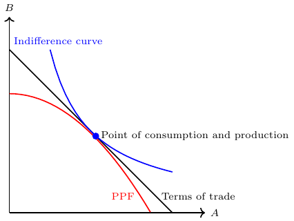
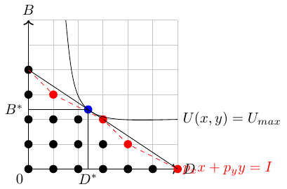
In microeconomics, utility maximization (in its simplest form when having just two goods) involves selecting a combination of two goods that satisfies two essential conditions, see Figure 10.1:

The chosen point of utility maximization must fall within the attainable region defined by the Production Possibility Frontier (PPF) or be affordable within the constraints of a given budget.
The selected point of utility maximization must lie on the highest indifference curve that is consistent with the first condition.

These conditions ensure that the consumer selects the optimal bundle of goods that maximizes their utility while taking into account the constraints imposed by production capabilities or budget limitations.

By analyzing production possibilities and individual preferences, economists gain insights into how consumers make choices, allocate resources, and achieve utility maximization. Understanding these concepts helps economists explore the trade-offs and decision-making processes that influence consumer behavior and shape market dynamics.

If you are not familiar with the basic principles of the production possibility frontier curve, indifference curves, and budget constraints, I recommend referring to Appendix A for a comprehensive overview. This section provides a detailed explanation and exploration of these concepts.

10.1.1 The role of income and budget

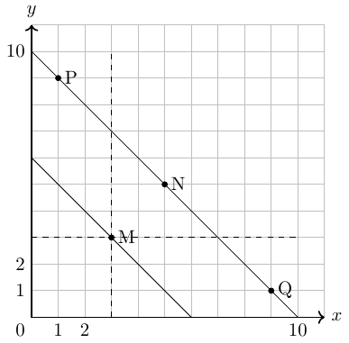
If income increases the budget constraint curve shifts outwards (to the right) as shown in Figure 10.2.

Figure 10.2: Impact of income change on consumption

The utility-maximizing choice on the original budget constraint is M. The dashed horizontal and vertical lines extending through point M allow you to see at a glance whether the quantity consumed of goods on the new budget constraint is higher or lower than on the original budget constraint. On the new budget constraint, a choice like N will be made if both goods are normal goods. If good $x$ is an inferior good, a choice like P will be made. If good $y$ is an inferior good, a choice like Q will be made.

10.1.2 The role of prices

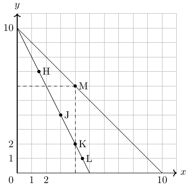
If price of one good increases then the budget constraint curve. When the price rises, the budget constraint shifts in to the left for that good.

Figure 10.3: Impact of price change on consumption

The dashed lines make it possible to see at a glance whether the new consumption choice involves less of both goods, or less of one good and more of the other. The new possible choices would be good $x$’s and more good $y$’s, like point H, or less of both goods, as at point J. Choice K would mean that the higher price of good $x$ led to exactly the same quantity of good $x$ being consumed, but fewer of good $y$. Choices like L are theoretically possible (if good $x$ are giffen goods) but highly unlikely in the real world, because they would mean that a higher price for goods $x$ means a greater quantity consumed of good $x$.

10.1.3 Substitution and income effect

When prices increase, individuals typically respond by reducing their consumption of the product with the higher price. This reaction is driven by two factors, both of which can occur simultaneously.

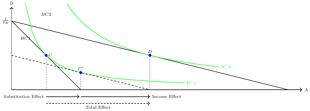
Figure 10.4: Impact of income change on consumption

The substitution effect occurs when a price change incentivizes consumers to consume less of a good with a relatively higher price and more of a good with a relatively lower price.

The income effect stems from the fact that a higher price effectively reduces the purchasing power of income (even if actual income remains the same). This reduction in purchasing power leads to a decrease in the consumption of the good, particularly when the good is considered normal.

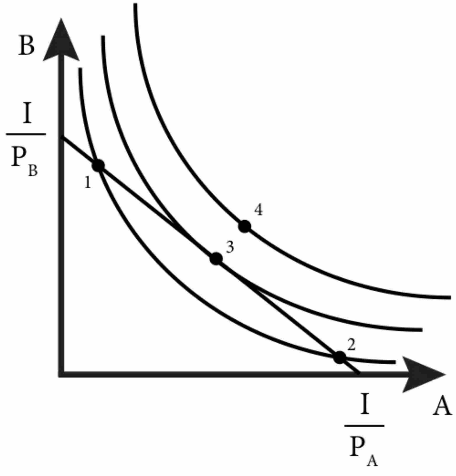
Figure 10.4 illustrates the Hicksian decomposition for a price reduction of good $A$, which affects the consumption of goods $A$ and $B$, shifting the consumption point from $C$ to $D$. The point $C'$ represents the hypothetical consumption point resulting from a rotated budget constraint that reflects the new price relationship.

Exercise 10.1 The graphical foundations of demand curves

A shift in the budget constraint means that when individuals are seeking their highest utility, the quantity that is demanded of that good will change. In this way, the logical foundations of demand curves—which show a connection between prices and quantity demanded—are based on the underlying idea of individuals seeking utility.

In Figure 10.5, two points of consumption are displayed, illustrating the optimal choices made by customers when faced with prices $p_x^1>p_x^2$. The objective of this exercise is to graphically derive the demand function for good $x$. To accomplish this, please provide a second two-dimensional plot below the existing graph, with the price of good $x$, $p_x$, represented on the y-axis.

Figure 10.5: Graphical derivation of the demand function

10.1.4 Consumption, production, and terms of trade

Market prices in a closed economy: The price relation of two goods, the so-called terms of trade, is determined by the slope of the Production Possibility Frontier (PPF) at the point where it is tangent to the indifference curve. This relationship highlights the trade-off between the two goods and their relative scarcity within a closed economy.

Utility maximizing production: The production point that maximizes utility is where the PPF is tangent to the price relation, that is, the terms of trade. This principle applies not only in a closed economy (autarky) but also under free trade (open economy). It implies that producers should allocate resources in a way that balances the trade-off between producing more of one good at the expense of another, while considering consumer preferences. Figure 10.1 depicts this.

10.2 Linear programming

Linear Programming is a common technique for decision making under certainty. It allows to express a desired benefit (such as profit) as a mathematical function of several variables. The solution is the set of values for the independent variables (decision variables) that serves to maximize the benefit or to minimize the negative outcome under consideration of certain limits, a.k.a. constraints. The method usually follows a four step procedure:

state the problem;
state the decision variables;
set up an objective function;
clarify the constraints.

Example: Consider a factory producing two products, product X and product Y. The problem is this: If you can realize $10.00 profit per unit of product X and $14.00 per unit of product Y, what is the production level of x units of product X and y units of product Y that maximizes the profit P each day? Your production, and therefore your profit, is subject to resource limitations, or constraints. Assume in this example that you employ five workers—three machinists and two assemblers—and that each works only 40 hours a week.¹

¹ The example is taken from Morse et al. (2014, p. 134f).

Morse, L. C., Babcock, D. L., & Murthy, M. (2014). Managing engineering and technology (Sixth Edition). Pearson.

Product X requires three hours of machining and one hour of assembly per unit.
Product Y requires two hours of machining and two hours of assembly per unit.

State the problem: How many of product X and product Y to produce to maximize profit?
Decision variables: Suppose x denotes the number of product X to produce per day and y denotes number of product Y to produce per day
Objective function: Maximize \[P = 10x + 14y\]
Constraints:

machine time=120h
assembling time=80h
hours needed for production of one good:

machine time: $x\rightarrow 3h$ and $y \rightarrow 2h$

assembling time: $x\rightarrow 1h$ and $y \rightarrow 2h$

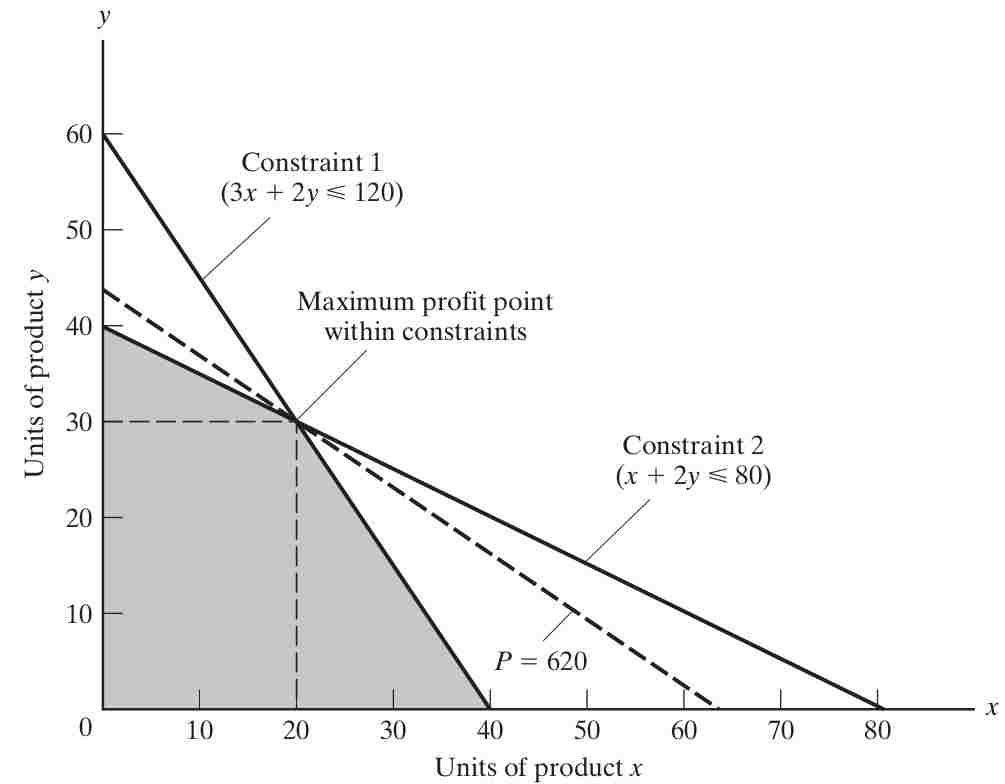
Thus, we get: \[3x + 2y \leq 120 \quad \Leftrightarrow y\leq 60-\frac{3}{2}x \quad \text{(hours of machining time)}\] \[x + 2y \leq 80 \quad \Leftrightarrow y \leq 40-\frac{1}{2}x \quad \text{(hours of assembly time)}\] Since there are only two products, these limitations can be shown on a two-dimensional graph Figure 10.6. Since all relationships are linear, the solution to our problem will fall at one of the corners.

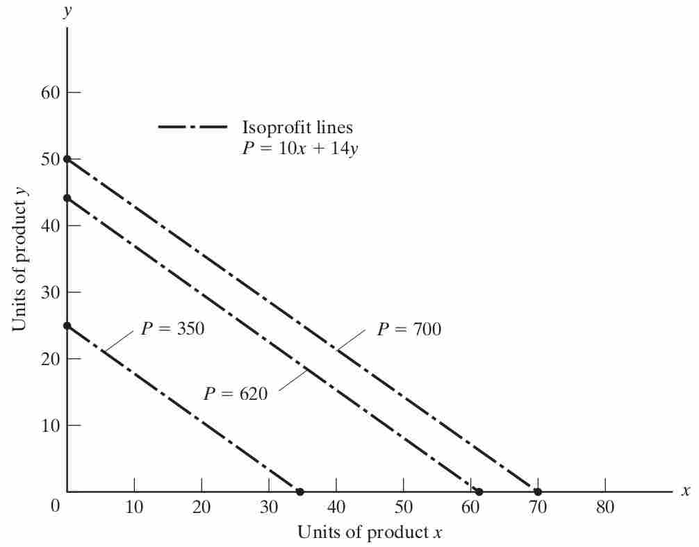
Figure 10.6: Linear program example: Constraints and solution

To draw the isoprofit function in a plot with the good $y$ on the y-axis and good $x$ on the x-axis, we can re-arrange the objective function to get \[y=\frac{1}{14}P-\frac{10}{14}x\] To illustrate the function let us consider some arbitrarily chosen levels of profit in Figure 10.7:

$350 by selling 35 units of X or 25 units of Y
$700 by selling 70 units of X or 50 units of Y
$620 by selling 62 units of X or 44.3 units of Y.

Figure 10.7: Linear program example: Isoprofit lines

To find the solution, begin at some feasible solution (satisfying the given constraints) such as $(x,y) = (0,0)$, and proceed in the direction of steepest ascent of the profit function (in this case, by increasing production of Y at $14.00 profit per unit) until some constraint is reached. Since assembly hours are limited to 80, no more than 80/2, or 40, units of Y can be made, earning $40 \cdot \$14.00$, or $560 profit. Then proceed along the steepest allowable ascent from there (along the assembly constraint line) until another constraint (machining hours) is reached. At that point, (x,y) = (20,30) and profit P = (20 * +10.00) + (30 * +14.00), or $620. Since there is no remaining edge along which profit increases, this is the optimum solution.

10.3 Lagrange multiplier method

The method outlined below requires an understanding of how to take derivatives of functions and solve systems of equations. If readers feel they need a refresher on these topics, I recommend consulting the lecture notes Calculus and Linear Algebra from Huber (2023).

Huber, S. (2023). Mathematics and statistics I: Calculus and linear algebra (lecture notes). online. https://raw.githubusercontent.com/hubchev/courses/main/pdfs/cla_A4.pdf

Figure 10.8: Joseph-Louis Lagrange (1736-1813)²

The decision-making process of consumers and producers lies at the core of microeconomic research and is of significant importance for managers. I will not go into detail here, but I will show some examples of how to come to a decision when certain information is given.

For a deeper understanding of the microeconomic preliminaries related to this topic, please read section Appendix A of the appendix.

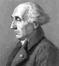
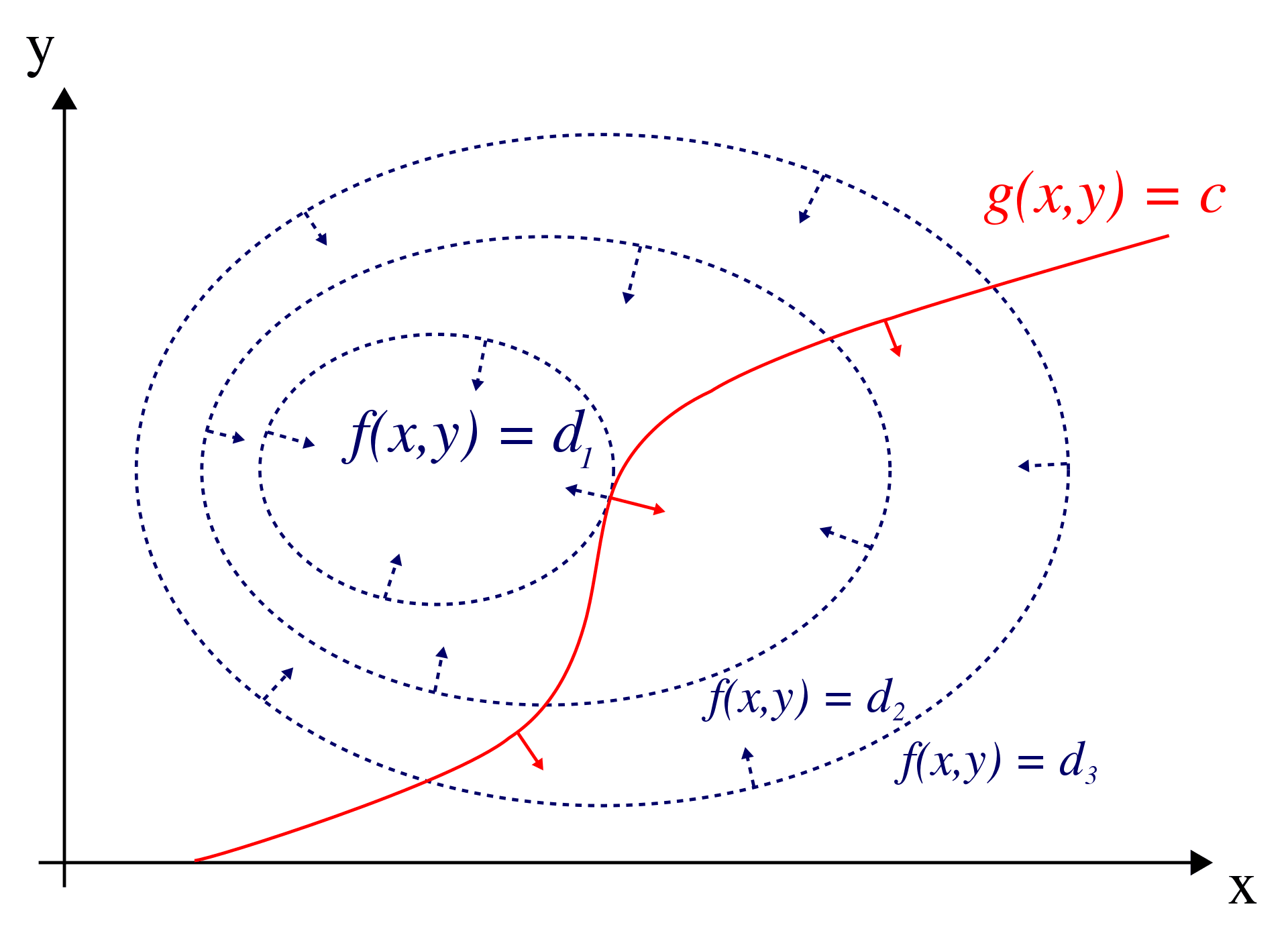
Figure 10.9: Contours of the function and the constraint in red

The Lagrange multiplier method, named after Joseph-Louis Lagrange (see Figure 10.8), is a strategy for finding the local maxima and minima of a function subject to constraints. The red curve in Figure 10.9 represents the constraint $g(x, y) = c$, while the blue curves depict contours of $f(x, y)$. The point where the red constraint tangentially intersects a blue contour represents the maximum of $f(x, y)$ along the constraint, as $d1 > d2$.

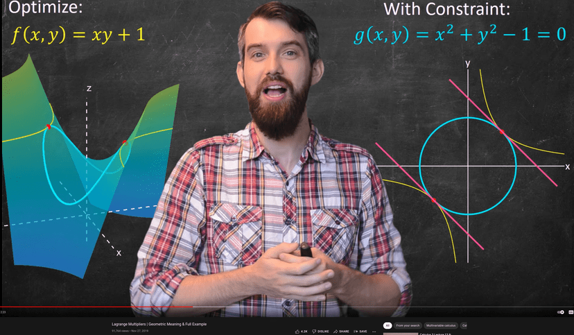
For a detailed visual explanation of the method, you can watch Dr. Trefor Bazett’s YouTube video on Lagrange Multipliers | Geometric Meaning & Full Example, see Figure 10.10.

Figure 10.10: Lagrange Multiplier graphically explained³

The Lagrange multiplier method, named after Joseph-Louis Lagrange, is a powerful technique for solving optimization problems with constraints. It allows us to find the local maxima and minima of a function subject to certain conditions. The method involves four key steps:

Step 1: Formulate the Problem

Define the problem you want to solve in mathematical terms. This includes specifying the objective function to be maximized or minimized and the constraints that need to be satisfied.

The problem that we want to solve can be written in the following way, \[ \begin{array}{ll} \max _{x, y} & F(x, y) \\ \text{ s.t. } & g(x, y)=0 \end{array} \] where $F(x, y)$ is the function to be maximized and $g(x, y)=0$ is the constraint to be respected. Notice that $\max _{x, y}$ means that we must solve (maximize) with respect to $x$ and $y$.

Step 2: Construct the Lagrangian

Create a new function called the Lagrangian by combining the objective function and the constraints using Lagrange multipliers. The Lagrangian introduces new variables, known as Lagrange multipliers, to account for the constraints. The Lagrangian, $\mathcal{L}$, is a combination of the functions that explain the problem: The $\lambda$ is called the Lagrange Multiplier. \[ \mathcal{L}(x, y, \lambda)=F(x, y)-\lambda g(x, y) \]

Step 3: Determine the First-Order Conditions

Differentiate the Lagrangian with respect to the variables of the problem (e.g., x and y) and the Lagrange multipliers. Set the partial derivatives equal to zero to obtain the first-order conditions. These conditions represent the necessary conditions for optimality.

Differentiate $\mathcal{L}$ w.r.t. $x, y,$ and $\lambda$ and equate the partial derivatives to 0: \[\begin{align*} \frac{\partial \mathcal{L}(x, y, \lambda)}{\partial x}=0 & \Leftrightarrow \frac{\partial F(x, y)}{\partial x}-\lambda \frac{\partial g(x, y)}{\partial x}=0 \\ \frac{\partial \mathcal{L}(x, y, \lambda)}{\partial y}=0 & \Leftrightarrow \frac{\partial F(x, y)}{\partial y}-\lambda \frac{\partial g(x, y)}{\partial y}=0 \\ \frac{\partial \mathcal{L}(x, y, \lambda)}{\partial \lambda}=0 & \Leftrightarrow g(x, y)=0 \end{align*}\]

Step 4: Solve the System of Equations

Solve the system of equations obtained from the first-order conditions to find the values of the variables and Lagrange multipliers that satisfy the optimality conditions. The solutions represent the optimal quantities that maximize or minimize the objective function subject to the given constraints.

By following these four steps, you can effectively apply the Lagrange multiplier method to various optimization problems with constraints. It provides a systematic approach to finding the optimal solutions while incorporating the necessary trade-offs imposed by the constraints.

10.4 Exercises

Exercise 10.2 Burgers and drinks

Suppose you are in a fast food restaurant and you want to buy burgers and some drinks. You have €12 to spend, a burger costs €3 and a drink costs €2.

Assume that you want to spend all your money and that you can only buy complete units of each products. What are the possible choices of consumption?
Given your utility function $U(x,y)=B^{0.6}D^{0.4}$ calculate for each possible consumption point your overall utility. How will you decide?
Assume that you want to spend all your money and that both products can be bought on a metric scale where one burger weights 200 grams and a drink is 200 ml. How much of both goods would you consume now? Hint: Use the Lagrangian multiplier method.⁴

Solution

In Figure 10.11, I marked all 19 possible bundles of burger and drinks of consumption. The budget constraint is shown by the solid line.

Figure 10.11: Possible consumption choices

We now should calculate the utility of all 19 points, but only the red dots denote choices that may yield an optimal utility. The best utility is achieved when we buy 2 burgers and 3 drinks:

\[U=2^{0.6}3^{0.4}=2.35\]

Solve:

\[ \mathcal{L}=B^{0.6}D^{0.4}+\lambda(3B+2D-12) \]

FOC: \[\begin{align*} 3B+2D-12&=0\\ 0.6B^{-0.4}D^{0.4}+3\lambda&=0\\ 0.4B^{0.6}D^{-0.6}+2\lambda&=0 \end{align*}\]

Solving the second and third FOC for $\lambda$ and substituting $\lambda$ gives:

\[B=D\]

which we can plug into the first FOC to obtain:

\[B^*=2.4 \quad \text{and} \quad D^*=2.4\]

⁴ Also see: http://www.sfu.ca/~wainwrig/5701/notes-lagrange.pdf

Exercise 10.3 Labor and machines

Suppose you rent a factory for a month to produce as many masks as possible. After you have paid the rent, you need to decide how many machines to buy and how many workers to hire for the given month.

What is the optimal amount of workers and machines to employ for the given month, if you assume the following:

$L$ denotes the number of workers
$K$ denotes the number of machines
$Q$ denotes the number of masks produced
$p_L$ denotes the price of a worker for a month
$p_K$ denotes the price of a machine for a month
$B$ denotes the money you can invest in the production of masks for the next month
$B = 216$
The production of masks can be explained by the following Cobb-Douglas production function: $Q = K^{0.4}L^{0.6}$
$p_L = 2$
$p_K = 8$

Solution

Set up Lagrangian: \[\mathcal{L} = K^{0.4}L^{0.6} - 216\lambda + 2\lambda L + 8\lambda K\]
FOC: \[\begin{align*} 0 &= 0.4K^{-0.6}L^{0.6} - 8\lambda \quad (*) \\ 0 &= 0.6K^{0.4}L^{-0.4} - 2\lambda \quad (**) \\ 0 &= 216 - 2L - 8K \quad (***) \\ \end{align*}\]
Solving (*) and (**) for $\lambda$ and substituting $\lambda$ gives us: \[\frac{1}{6}L = K \quad (****)\]
Plugging (****) into (***) yields: \[0 = 216 - 2L - 8\cdot\left(\frac{1}{6}L\right) \Rightarrow L = 64\frac{4}{5}\]
Using that result in (***) again, we get: \[216 - 2\cdot 64\frac{4}{5} + 8K \Rightarrow K = 10\frac{4}{5}\]

Thus, the optimal combination of inputs is $L = 64\frac{4}{5}$ and $K = 10\frac{4}{5}$.

Exercise 10.4 Consumption choice

Suppose you want to spend your complete budget of €30, \[I=30,\] on the consumption of two goods, $A$ and $B$. Further assume good $A$ costs €6, \[p_A=6,\] and good $B$ costs €4, \[p_B=4\] and that you want to maximize your utility that stems from consuming the two goods. Calculate how much of both goods to buy and consume, respectively, when your utility function is given as \[U(A,B)=A^{0.8}B^{0.2}\]

Solution

\[\begin{align*} \mathcal{L}&=A^{0.8}B^{0.2}+\lambda(6A+4B-30)\\ FOC: \frac{\partial \mathcal{L}}{\partial \lambda}&=6A+4B-30=0 \qquad (*)\\ \frac{\partial \mathcal{L}}{\partial A}&=0.8A^{-0.2}B^{0.2}+6\lambda=0 \qquad (**)\\ \frac{\partial \mathcal{L}}{\partial B}&=0.2A^{0.8}B^{-0.8}+4\lambda=0 \qquad (***) \end{align*}\] System of 3 equation with 3 unknowns can be solved in various ways. The easiest way is to solve () and (*) for $\lambda$ and substitute it out:

solve for $\lambda$ \[\begin{align*} -\frac{2}{15} A^{-0.2}B^{0.2}&=\lambda \qquad (**')\\ -\frac{1}{20} A^{0.8}B^{-0.8}&=\lambda \qquad (***')\\ \end{align*}\]
set both equations equal by substituting $\lambda$ and solve for $B$ \[\begin{align*} \frac{2}{15} A^{-0.2}B^{0.2}&= \frac{1}{20} A^{0.8}B^{-0.8}\\ B&=0.375A \qquad (****) %\\ \end{align*}\]
Now, plug in $(****)$ into $(*)$ to get a number for $A$ \[\begin{align*} 30&=6A+4\cdot 0.375 A\\ \Leftrightarrow 30&=7.5A\\ \Leftrightarrow A&=4 \end{align*}\]
Use $A=4$ in $(*)$ to get a number for $B$ \[\begin{align*} 30&=6\cdot 4+4 B\\ \Leftrightarrow 6&=4B\\ B&=\frac{6}{4}=1.5 \end{align*}\]

Thus, we’d consume 4 units of good A and 1.5 of good B.

Exercise 10.5 Cost-minimizing combination of factors

Using two input factors $r_1$ and $r_2$, a firm wants to produces a fixed quantity of a product, that is $x=20$. Given the production function \[ x=\frac{5}{4} r_1^{\frac{1}{2}} r_2^{\frac{1}{2}} \] and the factor prices \[ p_{r_1}=1 \quad \text{ and } p_{r_2}=4. \] calculate the cost-minimizing combination of factors ($r_1, r_2$).

Solution

\[ \mathcal{L}=r_1+4r_2+\lambda\left(\frac{5}{4}r_1^{\frac{1}{2}}r_2^{\frac{1}{2}}-20\right) \] Taking the FOC we get \[r_1=4r_2\] using that in the constraint, we get $r_1=32$ and $r_2=8$.

Also see which uses this tool:

Exercise 10.6 Lagrange with n-constraints

Write down the Lagrangian multiplier for the following minimization problem:

Minimize $f(\mathbf{x})$ subject to: \[\begin{aligned} g_1(\mathbf{x})&=0 \\ g_2(\mathbf{x})&=0\\ &\vdots\\ g_n(\mathbf{x})&=0,\end{aligned}\] where $n$ denotes the number of constraints.

Solution

\[ \mathcal{L}(x_1, \dots, x_m, \lambda_i, \dots, \lambda_n)=f(\mathbf{x})+\lambda_1 g_1(\mathbf{x})+\lambda_2 g_2(\mathbf{x})+\ldots+\lambda_n g_n(\mathbf{x}) \] The points of local minimum would be the solution of the following equations: \[\begin{align*} \frac{\partial \mathcal{L}}{\partial x_{j}} &=0 \quad \forall j=1 \dots m \\ g_i(\mathbf{x}) &=0 \quad \forall i=1\dots n \end{align*}\]

Exercise 10.7 Derivation of demand function using the Lagranian multiplier

A representative consumer has on average the following utility function: $U=x y,$ and faces a budget constraint of $B=P_{x} x+P_{y} y,$ where $B, P_{x}$ and $P_{y}$ are the budget and prices, which are given. Solve the following choice problem:

Maximize $U=x y$ s.t. $B=P_{x} x+P_{y} y$.

Solution

The Lagrangian for this problem is \[ Z=x y+\lambda\left(P_{x} x+P_{y} y-B\right) \] The first order conditions are \[ \begin{array}{l} Z_{x}=y+\lambda P_{x}=0 \\ Z_{y}=x+\lambda P_{y}=0 \\ Z_{\lambda}=-B+P_{x} x+P_{y} y=0 \end{array} \]

Solving the first order conditions yield the following solutions

\[ x^{M}=\frac{B}{2 P_{x}} \quad y^{M}=\frac{B}{2 P_{y}} \quad \lambda=\frac{B}{2 P_{x} P_{y}} \] where $x^{M}$ and $y^{M}$ are the consumer’s demand functions.

Exercise 10.8 Cobb-Douglas and demand

A consumer who has a Cobb-Douglas utility function $u(x, y)=A x^{\alpha} y^{\beta}$ faces the budget constraint $p x+q y=I$, where $A, \alpha, \beta, p,$ and $q$ are positive constants. Solve the problem:

\[ \begin{array}{lll} \max A x^{\alpha} y^{\beta} & \text { subject to } & p x+q y=I \end{array} \]

Solution

The Lagrangian is \[ \mathcal{L}(x, y)=A x^{\alpha} y^{\beta}+\lambda(p x+q y-I) \]

Therefore, the first-order conditions are \[ \begin{aligned} \mathcal{L}_{x}^{\prime}(x, y)=A \alpha x^{\alpha-1} y^{\beta}+\lambda p &=0 \qquad (*)\\ \mathcal{L}_{y}^{\prime}(x, y)=A x^{\alpha} \beta y^{\beta-1}+\lambda q &=0 \qquad (**)\\ p x+q y-I &=0 \qquad (***) \end{aligned} \]

Solving $(*)$ and $(**)$ for $\lambda$ yields \[ \lambda=\frac{A \alpha x^{\alpha-1} y^{\beta-1} y}{p}=\frac{A x^{\alpha-1} x \beta y^{\beta-1}}{q} \] Canceling the common factor $A x^{\alpha-1} y^{\beta-1}$ from the last two fractions gives \[ \frac{\alpha y}{p}=\frac{x \beta}{q} \] and therefore \[ q y=p x \frac{\beta}{\alpha} \] Inserting this result in $(***)$ yields \[ p x+p x \frac{\beta}{\alpha}=I \] Rearranging gives \[ p x\left(\frac{\alpha+\beta}{\alpha}\right)=I \] Solving for $x$ yields the following demand function \[ x=\frac{\alpha}{\alpha+\beta} \frac{I}{p} \] Inserting \[ p x=q y \frac{\alpha}{\beta} \] in $(***)$ gives \[ q y \frac{\partial}{\beta}+q y=I \] and therefore the _demand function} \[ y=\frac{\beta}{\alpha+\beta} \frac{I}{q} \]

Exercise 10.9 Understanding indifference curves and budget constraints

Which indifference curve in the figure on the right represents the highest utility level? Explain your decision.
Suppose two goods are perfect substitutes. Two goods are substitutes if they can be used for the same purpose or provide the same utility to the consumer. Draw the indifference curves for perfect substitutes.
Suppose two goods are perfect complements. Two goods are complements if they go well together and the demand for one good is related to the demand for another good. A perfect complement is a good that must be consumed together with another good. Draw the indifference curves for perfect complements.
Suppose you have a fixed income $I=10$ that you can spend on consuming two goods $x, y$ at certain prices $p_x=1, p_y=1$. Draw the budget line consisting of all possible combinations of two goods that a consumer can buy at certain market prices by allocating his income. Using indifference curves, sketch what each consumer should consume to maximize utility.

Solution

$IC_3$ represents the highest level of utility. $IC_1$ represents the lowest level of utility.
Task solved in class.
Task solved in class.
The budget line can be sketched into a y-x plot by solving $p_xx+p_yy=I$ for y: \[y=\frac{I}{p_y}-\frac{p_x}{p_y}x\]

Exercise 10.10 Utility maximization

Figure 10.12 stems from Emerson (2019, ch. 4). Use the following sentences to describe the respective points in the figure.

Optimal bundle.
Can do better by trading some B for some A.
Can do better by trading some B for some A.
Unaffordable.

Please find solutions to the exercise in Emerson (2019, ch. 4).

Emerson, P. M. (2019). Intermediate microeconomics (O. S. University, Ed.; 1st edition). Open Educational Resources. https://open.oregonstate.education/intermediatemicroeconomics