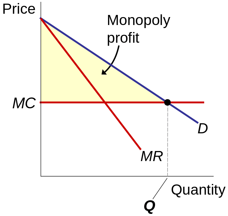
14 Monopoly

A monopolist is a firm that is the only provider of a good or service. There is no close substitute to it. The ability of a monopolist to raise its price above the competitive level by reducing output is known as market power. This implies a loss of total welfare. In contrast with a perfectly competitive firm which faces a perfectly elastic demand (taking price as given), a monopolist faces the market demand. As a consequence, a monopolist has the power to set the market price. While we can consider a competitive firm as a price taker, a monopolist is price decision-maker or price setter. Firms that have to face fierce competition are more like price takers as they cannot set the price above the market price. If firms in perfect competition would set the price higher, all consumers would simply stop buying from that particular firm. That is not the case for a firm with market power, that is, a firm that has a product with unique features no other competitor has to offer.

14.1 Revenue function

There are two types of constraints that restrict the behavior of a monopolist (and any other firm):

Technological constraints summarized in the cost function \(C(x)\).
Demand constraints: \(x(p)\).

Thus, we can write the revenue (or profit) function of the monopolist in two alternative ways:

Either by using the demand function: \[ \pi(p) = px(p) - C(x(p)) \]
Or by using the inverse demand function: \[ \pi(x) = p(x)x - C(x) \]

The demand, \(x(p)\), and the inverse demand, \(p(x)\), represent the same relationship between price and demanded quantity from different points of view. The demand function is a complete description of the demanded quantity at each price, whereas the inverse demand gives us the maximum price at which a given output \(x\) may be sold in the market.

14.2 Revenue and price relationship

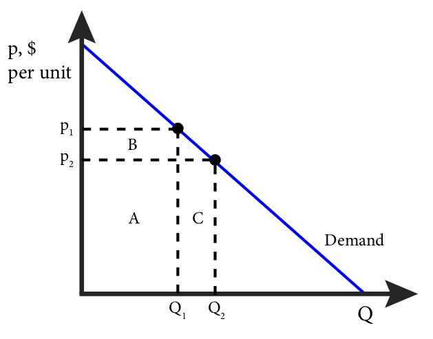
Thus, an increase in production by a monopolist has two opposing effects on revenue:

A quantity effect: one more unit is sold, increasing total revenue by the price at which the unit is sold.
A price effect: in order to sell the last unit, the monopolist must cut the market price on all units sold. This decreases total revenue.

The two effects are shown in figure Figure 14.1: At price \(p_1\), the total revenue is \(p_1 \cdot Q_1\), which is represented by the areas A+B. At price \(p_2\), the total revenue is \(p_2 \cdot Q_2\), which is represented by the areas A+C. Area A is the same for both, so the marginal revenue is the difference between B and C or C-B. Note that area C is the price, \(p_2\), times the change in quantity, \(Q_2 - Q_1\), or \(p \Delta Q\); and area B is the quantity, \(Q_1\), times the change in price, \(p_2 - p_1\), or \(\Delta p \cdot Q\). Since \(p_2 - p_1\) is negative, the change in total revenue is C-B or: \(\Delta TR = p \Delta Q + \Delta p \cdot Q\). Dividing both sides by \(\Delta Q\) gives us an expression for marginal revenue:

\[ MR = \frac{\Delta TR}{\Delta Q} = \underbrace{p}_{\text{quantity effect}} + \underbrace{Q \frac{\Delta p}{\Delta Q}}_{\text{price effect}} \]

14.3 Profit-maximizing level of output

To find the profit-maximizing price and quantity, respectively, we should look at the first-order conditions:

\[\begin{align*} \max_{p} \pi (p) \equiv& \max_{p} \quad px(p) - C(x(p))\\ \frac{\partial \pi (p)}{\partial p} =& \pi ' (p) = x(p) + px'(p) - C'(x(p))x'(p) \overset{!}{=} 0 \end{align*}\]

\[\begin{align*} \max_{p} \pi (x) \equiv& \max_{x} \quad p(x)x - C(x)\\ \frac{\partial \pi (x)}{\partial x} =& \pi ' (p) = \underbrace{p(x)}_{\text{quantity effect}} + \underbrace{xp'(x)}_{\text{price effect}} - C'(x) \overset{!}{=}& 0\\ \Rightarrow \underbrace{p(x) + xp'(x)}_{\text{marginal revenue}} =& \underbrace{C'(x)}_{\text{marginal costs}}\\ \Rightarrow MR =& MC \end{align*}\]

At the profit-maximizing level of output, marginal revenue equals marginal cost, that is, an infinitesimal change in the level of output changes revenue and cost equally. In other words, an infinitesimal increase in the level of output increases revenue and cost by the same amount, and an infinitesimal decrease in the level of output reduces revenue and cost by the same amount.

Thus, we can determine a monopoly firm’s profit-maximizing price and output by following three steps:

Determine the demand, marginal revenue, and marginal cost curves.
Select the output level at which the marginal revenue and marginal cost curves intersect.
Determine from the demand curve the price at which that output can be sold.

14.4 Price effect of a monopoly

Due to the price effect of an increase in output, the marginal revenue curve of a firm with market power always lies below its demand curve. So, a profit-maximizing monopolist chooses the output level at which marginal cost is equal to marginal revenue—not equal to price. As a result, the monopolist produces less and sells its output at a higher price than a perfectly competitive industry would. It earns a profit in the short run and the long run.

14.5 Welfare

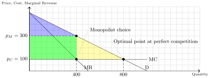
As illustrated in Figure Figure 14.2, the price-setting behavior of a monopolist typically leads to a reduction in overall welfare: The shaded green area represents the monopoly profit, and the blue area denotes the consumer surplus, the sum of both constitute the total welfare. The yellow triangle represents the deadweight loss, indicating the welfare that is lost due to the monopolist producing fewer goods at a higher price than in a competitive market. The horizontal line at \(p=100\) represents the marginal costs (MC).

Figure 14.2: Price setting of a monopolist

14.6 Price elasticity and market power

We know that the demand elasticity of price can be measured with:

\[ \frac{\triangle p/\bar{p}}{\triangle x / \bar{x}}. \]

Using differential calculus, the point-price elasticity of demand (PPD) can be written as:

\[ PPD = \frac{\partial p(x)}{\partial x} \cdot \frac{x}{p(x)} \]

This can also be expressed as:

\[ PPD = p'(x) \frac{x}{p(x)} = x \frac{p'(x)}{p(x)} \]

Thus, if \(PPD = 0\), the price does not change if a single firm increases its quantity sold on the market. That means the firms are price takers, and their quantity sold has no impact on the price. If firms, however, have market power, \(PPD < 0\), which means that if a firm increases the quantity on the market, the price must fall. The PPD can hence be interpreted as an indicator of the market power of firms.

14.7 Marginal revenue and price elasticity

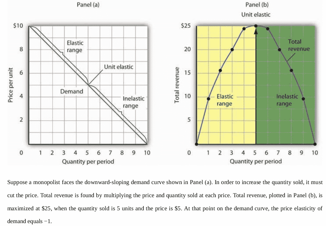
Now, plugging the PPD into the MR function, we can show that MR is equal to zero when we have a unit demand elasticity, PPD, of \(-1\):

\[ MR = p(x) + xp'(x) = p(x)\left(1 + x\frac{p'(x)}{p(x)}\right) = p(x)\left(1 + PPD\right) \]

Also see figure Figure 14.3. In the monopoly output, marginal revenue and marginal cost are equal:

\[ MC = p(x) \cdot \left(1 + PPD\right) \]

Figure 14.3: Price setting of a monopolist²

14.8 Lerner index

The Lerner index is a measure of monopoly power, which equals the markup over marginal cost as a percentage of price. To obtain the Lerner index of monopoly power (or market power), let us rearrange \(MC = p(x) \cdot \left(1 + PPD\right)\) as follows:

\[ \frac{MC - p(x)}{p(x)} = PPD = \text{Lerner Index} \]

If a firm does not have market power (\(PPD = 0\)), its price equals the marginal cost. When a firm’s market power is high (up to \(|PPD| = \infty\)), the higher the markup that a firm sets. In perfect competition, since \(p\) and MC are equal, the Lerner Index is 0. A pure monopolist, on the other hand, can theoretically charge an infinite markup, which leads us to a Lerner index of 1.

Exercise 14.1 Marginal revenue and total revenue

Show the relationship between a linear demand curve and the marginal revenue curve in one panel and the relationship of the quantity sold and the total revenue in another panel. What characterizes the price of a profit maximizing monopolist?

Solution

See: chapter 15.2 Profit Maximization for Monopolists of Emerson (2019), see: here.

Exercise 14.2 How to maximize profits

A company sold a quantity of 750 goods ((Q_{t=1}=750)) in January ((t=1)), at a price of 45 € ((P_{t=1}=45)). In February ((t=2)), they reduced the price to 40 Euro ((P_{t=2}=40)) and sold 800 goods ((Q_{t=2}=800)). Now answer the following questions knowing that the total costs had been 26,500 € in January and 28,000 € in February.

Calculate the price elasticity of demand at the current prices.
Derive the demand function.
Derive the cost function.
Derive the revenue function.
Derive the marginal revenue function.
Derive the marginal cost function.
Calculate the profit-maximizing price and output.
Calculate the amount of profit in January, February, and what the company can expect by setting the prices profit-maximizing.

Solution

The price elasticity of demand (PED) is given by: \[PED=\frac{17}{31} \approx 0.5483\]
The demand function can be derived using the point-slope formula and one sales point: \[P - 40 = -\frac{1}{10}(Q - 800) \Rightarrow P = 120 - \frac{1}{10}Q \Rightarrow Q = 1200 - 10P\]
Total costs (TC) are given by: \[TC = FC + VC = FC + MC \cdot Q.\] Solving the system of equations: \[26500 = FC + 750 \cdot MC\] \[28000 = FC + 800 \cdot MC\] we find that (MC = 30) and (FC = 4000). The cost function is: \[TC = 4000 + 30 \cdot Q.\]
The revenue function is given by: \[TR = P \cdot Q(P).\] Plugging the demand function in gives: \[TR(Q) = 120Q - \frac{1}{10}Q^2.\]
The marginal revenue function is: \[\frac{\partial TR(Q)}{\partial Q} = 120 - \frac{2}{10}Q.\]
The marginal cost function is: \[MC = 30\] (as found in step 3).
Setting (MC = MR), we find the optimal quantity: \[30 = 120 - \frac{2}{10}Q \Rightarrow Q^* = 450.\] Plugging (Q^) into the demand function, we find the optimal price: \[P^ = 120 - \frac{1}{10} \cdot 450 = 75.\]
Profit (\(\pi\)) is given by \(\pi = TR - TC\): \[\pi_{t=1} = 1200 \cdot 75 - 10 \cdot 75^2 - 4000 - 30 \cdot 750 = 7250\] \[\pi_{t=2} = 1200 \cdot 75 - 10 \cdot 75^2 - 4000 + 30 \cdot 800 = 4000\] \[\pi_{t=3} = 12\]

14.9 Monopoly and price discrimination

Discrimination is the practice of treating people differently based on some (irrelevant) characteristic, such as race or gender. It is important to actively fight discrimination whenever it is observed. However, the concept of discrimination takes a different form when it comes to price discrimination, which is a business practice involving the sale of the same goods at different prices to different buyers. This practice can be commonly seen in special offers tailored for students or retired individuals.

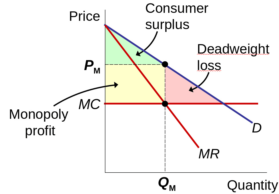
One of the key factors utilized in price discrimination is the willingness to pay (WTP) of individuals. By charging a higher price to buyers with a higher WTP, a firm can maximize its profit. Moreover, and that is kind of surprising, it also comes with a increase in social welfare as is shown in figure Figure 14.5 and figure Figure 14.5. In Figure 14.5, the monopolist charges the same price (PM) to all buyers. A deadweight loss results. In Figure 14.5, however, the monopolist produces the competitive quantity but charges each buyer his or her WTP. This is called perfect price discrimination. The monopolist captures all consumer surplus as profit. But there is no deadweight loss.

Figure 14.4: Monopoly without price discrimination and welfare

Figure 14.5: Monopoly with price discrimination and welfare

In the real world, price discrimination is a common phenomenon, but achieving perfect price discrimination is highly challenging. This is primarily because no firm possesses complete knowledge of every buyer’s willingness to pay (WTP), and buyers typically do not disclose this information to sellers. Consequently, firms often divide customers into groups based on observables that are likely correlated with their WTP.