15 Regional (preliminary)

15.1 Von Thünen model of land use

The classical model of spatial organization of the economy stems Heinrich von Thünen (1783-1850). The model focuses on agriculture as this was the dominant use of land at the time. However, the fundamental ideas of the model can be applied to various industries. The model can be described as follows: Assume a focal point of demand for agricultural goods (e.g., the marketplace of a large city). Differences in soil quality in the agricultural periphery of the considered city are neglected. The demand is differentiated. That means, various goods such as grains, dairy products, meat, timber, vegetables are required to satisfy the needs of the people. The goods differ in terms of

the market price they can achieve,
the assumed constant marginal production costs \((c_i)\),
the revenue per unit of land, and
in terms of their transportability, that is, each good has different specific transport costs \((\theta_i)\).

All mentioned variables are exogenously given. In particular, the model is based on the following assumptions:

Point-centered demand for all goods \(i\).
Different production methods possible, each with constant (marginal) production costs \(c_i\).
Homogeneous Space: The agricultural land surrounding the central marketplace is assumed to be uniform and homogeneous in terms of soil fertility, climate, and other relevant factors.
Given market prices for the individual products \(p_i\)
Producers supply the market and have linear product-specific transportation costs \((\theta_i)\).
Perfect competition: The model assumes perfect competition among farmers for the available land (free market access). That implies that they have full knowledge of market conditions and make rational decisions.

To analyze the model, let us start by considering the restriction to a single land use. The key idea is that the rent price for a unit of land arises from the net yield that this unit of land enables under that particular land use. However, since both production costs and distance-dependent transport costs need to be subtracted from the gross yield to determine the net yield, it follows that land rent is determined by the distance from the center. Under a given land use, the value of an agricultural area is significantly influenced by its distance from the marketplace.

Formally, the land rent for land use for production of good \(i\), depending on the distance \(x\) from the marketplace, is given by:

\[ r_i(x) = q_i(p_i - c_i - \theta_i \cdot x) \]

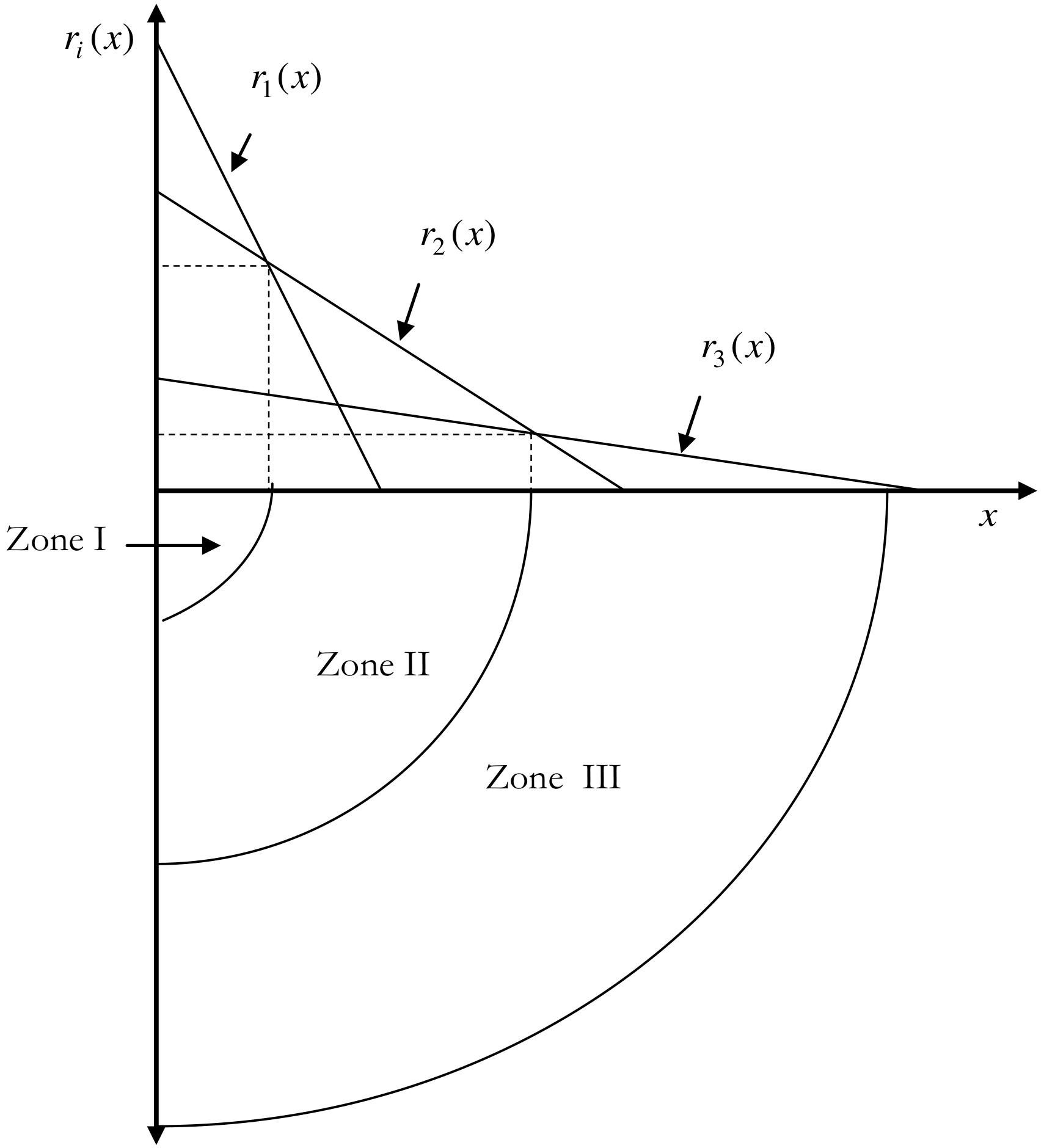
The land rent increases with the quantity demanded \((q)\) and the price of the good, and it decreases with the marginal production costs \((c)\), the specific transportation costs \((\theta)\), and the distance \((x)\) from the marketplace. The typical shape of a rent curve, with \(r\) on the y-axis and \(x\) on the x-axis, is a linearly decreasing curve. Its slope is determined by the expression \(-q_i \theta_i\). Therefore, the steeper the specific transportation costs, the steeper the curve.

Suppose, different land uses are allowed. By varying the price, revenue, and cost parameters in the equation above, different rent curves with varying locations and slopes emerge for different land uses. The interesting question now is: How high will the market rent be?

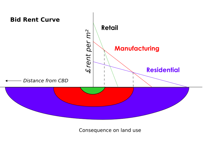
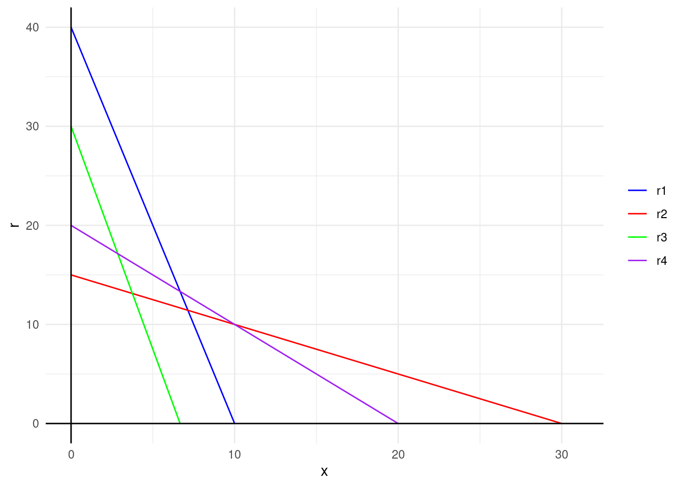
Thünen provides a clear answer to this question: Competition among land tenants will ensure that in a specific distance zone around the center, the production method with the highest net yield in that zone will prevail. In other words, the market rent curve (or bid rent curve) is the upper envelope of all rent curves for specific production methods. The situation is illustrated in figure @ref(fig:thuenen) and @ref(fig:thuenen2) for three different production methods. The intersections of the market rent curves determine the shifts in production zones.

(#fig:thuenen) Thünen’s rings of land use

This model is also known as the Bid rent theory. A short but nice explanation of the model can be found on Wikipedia, see here.

Exercise 15.1 Agricultural land use

In the vicinity of an agglomeration center, four different agricultural land use forms are possible. We have information about the specific yield per unit of land (q_i), the (constant) marginal costs (c_i), the specific transportation costs (_i), and the price (p_i) that can be achieved for a unit of the respective product in the center.

Where do we see which land use form?

	Production Form	Production Form	Production Form	Production Form
(i)	1	2	3	4
(q_i)	10	5	30	20
(p_i)	5	5	2	6
(c_i)	1	2	1	5
(_i)	0.4	0.1	0.15	0.05

Exercise 15.2 Business location model

The Thünenian approach is intended to be applied to a business location model. The customer frequency, depending on the distance \(x\) from the center, can be approximated by the following function:

[ f(x)i = A{0} e^{-a x} ]

The probability of sale per square meter for business type \(i\) is denoted by \(\lambda_i\). The business types also differ in terms of profit margin and fixed costs. Describe the market rent curve and show which business type will dominate in each location. What effects does an increase in the parameter \(a\) have? What about an increase in \(A_0\)? Interpret the changes in parameters and the results from an economic perspective.

15.2 Launhardt/Hotelling location model

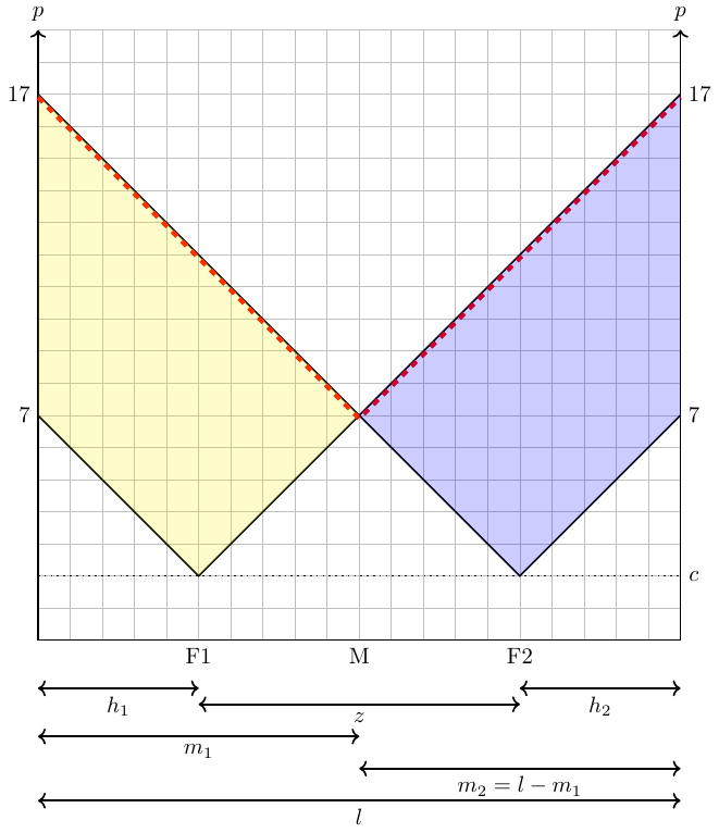
Consider a scenario where two firms, i.e., \(i={F1;F2}\), have the option to establish their locations along a linear market, such as a street or a beach. These firms can relocate without incurring any costs and sell an identical product at the same price. Consequently, the only means of competition available to them is by strategically selecting their respective locations. Moreover, assume that customers are uniformly distributed throughout the market, and each customer is willing to purchase one unit of the product up to a certain price, denoted as \(\bar{p}\). The cost of transportation is the same for both firms and is proportional to the distance between the firm and the customer.

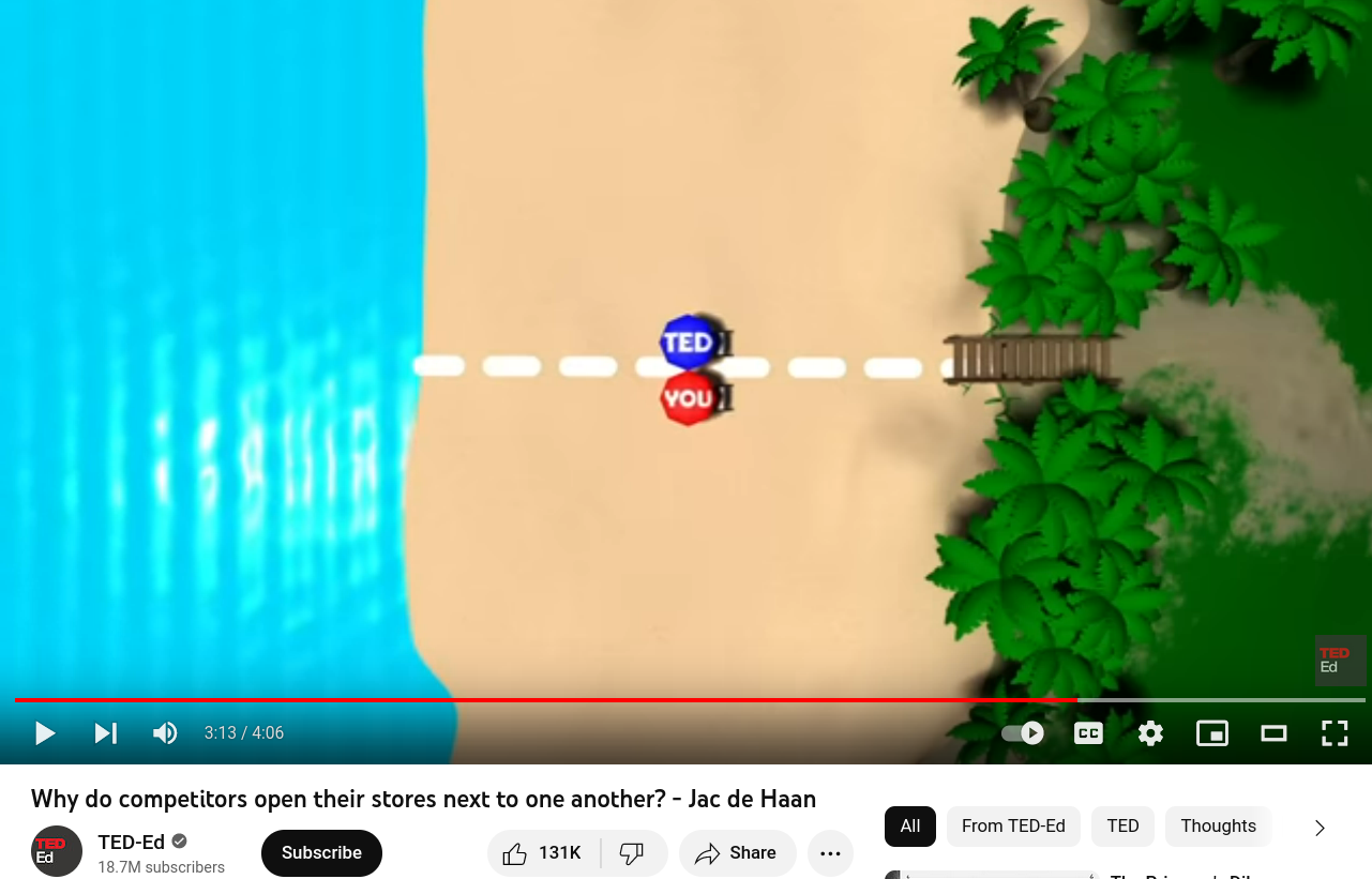
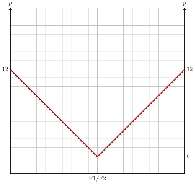
If we assume that the transportation costs are equal for both firms and that the market has a finite size, the firms will eventually position themselves at the center of the market with no empty space between them. The rationale and dynamics behind this behavior are clearly explained in the YouTube clip of TED-Ed Why do competitors open their stores next to one another? - Jac de Haan, see figure @ref(fig:hotelling). I highly recommend watching the clip.

(#fig:hotelling) YouTube clip of TED-Ed and Jac de Haan²

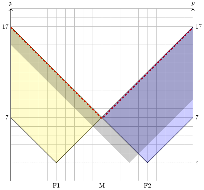
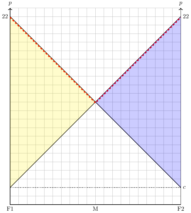
If we assume that the transportation costs can vary between the two firms, things became a bit more complicated. Let us define transportation costs for a firm as \(\theta_i=a_i d(x)\), where \(d(x)\) represents the distance between the company and the respective costumer and \(a_i\) is firm-specific costs of transportation. Let us further assume competition and loosen the assumption of fixed prices: Firms can set prices but they need to charge the price of the good, \(p\), plus their costs of transporting the good to the costumer. Thus, the price of a good a firm needs to charge in order not to make deficits is \[ p^{min}(x)=c+\theta_i=c+a_i d(x) \]

If we assume that the transport costs are the same for both firms and that the market is limited in size, the firms will end up at the center of the market with no space inbetween them. However, there is always an incentive to deviate from that minimum of spatial differentiation. However, the dynamic is kind of strange as we can show in the following four figures.