9 Finance

You are financially literate if you understand and manage personal finances effectively. It involves having a basic understanding of financial concepts, such as budgeting, saving, investing, and managing debt. Financial literacy also includes knowledge of financial products and services, such as bank accounts, credit cards, loans, and insurance. Being financially literate means having the skills and knowledge to make informed financial decisions, and being able to assess risks and opportunities when it comes to managing money. It is an important life skill that can help individuals achieve their financial goals, build wealth, and avoid financial pitfalls.

Being better-educated was always associated with having more financial knowledge (Figure 1) across the countries we examined,3 yet we also found that education is not enough. That is, even well-educated people are not necessarily savvy about money.

Unfortunately, financial illiteracy is widespread. While being better-educated is associated with making better financial decisions on average, “even well-educated people are not necessarily savvy about money” (Mitchell & Lusardi, 2015, p. 3).

There are various attempts to assess the levels of financial literacy. See https://www.oecd.org/finance/financial-education/measuringfinancialliteracy.htm for example.

Exercise 9.1 S&P Global FinLit Survey

One example of a comprehend way to measure financial literacy stems from the Standard & Poor`s Ratings Services Global Financial Literacy Survey (see Klapper & Lusardi, 2020). They ask the following multiple-choice questions:

Suppose you have some money. Is it safer to put your money into one business or investment, or to put your money into multiple businesses or investments?
1. One business or investment
2. Multiple businesses or investments
3. Don`t know
4. Refused to answer
Suppose over the next 10 years the prices of the things you buy double. If your income also doubles, will you be able to buy less than you can buy today, the same as you can buy today, or more than you can buy today?
1. Less
2. The same
3. More
4. Don`t know
5. Refused to answer
Suppose you need to borrow $100. Which is the lower amount to pay back: $105 or $100 plus 3%?
1. $105
2. $100 plus 3%
3. Don`t know
4. Refused to answer
Suppose you put money in the bank for 2 years and the bank agrees to add 15% per year to your account. Will the bank add more money to your account the second year than it did the first year, or will it add the same amount of money both years?
1. More
2. The same
3. Don`t know
4. Refused to answer
Suppose you had $100 in a savings account and the bank adds 10% per year to the account. How much money would you have in the account after 5 years if you did not remove any money from the account?
1. More than $150
2. Exactly $150
3. Less than $150
4. Don`t know
5. Refused to answer

These questions cover four fields of financial literacy, i.e., risk diversification, inflation and purchasing power, numeracy (simple calculations related to interest rates), and compound interest (interest payments increase exponentially over time). Knowledge in these concepts is important to make good financial decisions and to manage risk.

Try to answer these quesions and compare your performance with the results shown in Klapper & Lusardi (2020).

Solution

Correct answers are:

Klapper, L., & Lusardi, A. (2020). Financial literacy and financial resilience: Evidence from around the world. Financial Management, 49(3), 589–614. https://onlinelibrary.wiley.com/doi/full/10.1111/fima.12283

Exercise 9.2 The three questions

Referring to Mitchell & Lusardi (2015), only 21.7% of individuals in Germany with a lower secondary education and 72% of those with tertiary education can correctly answer all three of the following questions. Try it yourself!

Suppose you had $100 in a savings account and the interest rate was 2% per year. After 5 years, how much do you think you would have in the account if you left the money to grow?
1. More than $102
2. Exactly $102
3. Less than $102
4. Do not know
5. Refuse to answer
Imagine that the interest rate on your savings account was 1% per year and inflation was 2% per year. After 1 year, how much would you be able to buy with the money in this account?
1. More than today
2. Exactly the same
3. Less than today
4. Do not know
5. Refuse to answer
Please tell me whether this statement is true or false: “Buying a single company’s stock usually provides a safer return than a stock mutual fund.”
1. True
2. False
3. Do not know
4. Refuse to answer

These three questions are designed to measure Lusardi & Mitchell (2014) reports that in many countries the financial illiteracy is considerably high as the following table shows:

Financial literacy around the World
	% all correct	% none correct
Germany	57	10
Netherlands	46	11
United States	35	10
Italy	28	20
Sweden	27	11
Japan	27	17
New Zealand	27	4
Russia	3	28

Solution

Correct answers are:

Lusardi, A., & Mitchell, O. S. (2014). The economic importance of financial literacy: Theory and evidence. Journal of Economic Literature, 52(1), 5–44.

Mitchell, O. S., & Lusardi, A. (2015). Financial literacy and economic outcomes: Evidence and policy implications. The Journal of Retirement, 3, 1, 107–114.

9.1 Simple financial mathematics

I discuss financial mathematics in the following chapter just briefly. If you want to gather a deeper understanding, I recommend the open textbook of Dahlquist et al. (2022) or the respective chapters of Wilkinson (2022).

Dahlquist, J., Knight, R., Adams, A. S., Bacon, C. J., Cooper, S. T., Griffin, M. P., Higgins, K. C., & Musolino, L. (2022). Principles of finance. OpenStax. https://biz.libretexts.org/Bookshelves/Finance/Principles_of_Finance_(OpenStax)

Wilkinson, N. (2022). Managerial economics problem-solving in a digital world (2nd ed.). Cambridge University Press.

9.1.1 Simple Interest

Suppose $r$ denotes annual interest rates, $P$ denotes the initial deposit which earns the interest, $A$ denotes the value of the deposit at the end of an investment. Then, the relationship of these for a single year is

\[ A=P+Pr=P(1+r) \]

and for many years, $t$, it is

\[ A=P(1+rt) \]

which is the simple interest formula. It gives the amount due when the annual interests does not become part of the deposit $P$.

9.1.2 Compound interest

If the annual interest, $P(1+r)$, is added to $P$, we need a formula that takes this into account, and for two periods this is

\[ A=P\cdot [(1+r)\cdot(1+r)]=P(1+r)^2 \]

and for t periods

\[ A=P(1+r)^t. \]

Compound interest is the addition of interest to the principal sum of a loan or deposit, or in other words, interest on principal plus interest. It is the result of reinvesting interest, or adding it to the loaned capital rather than paying it out, or requiring payment from borrower, so that interest in the next period is then earned on the principal sum plus previously accumulated interest.

\[ A=P\left(1+\frac{r}{n}\right)^{nt} \]

Example

Suppose a principal amount of $1,500 is deposited in a bank paying an annual interest rate of 4.3%, compounded quarterly. Then the balance after 6 years is found by using the formula above, with $P = 1500$, $r = 0.043$ (4.3%), $n = 4$, and $t = 6$:

\[ A=1500\times\left(1+\frac{0.043}{4}\right)^{4\times 6}\approx 1938.84 \]

So the amount $A$ after 6 years is approximately $1,938.84.

Subtracting the original principal from this amount gives the amount of interest received: $1938.84-1500=438.84$

9.1.3 Continuously compounded interest

As $n$, the number of compounding periods per year, increases without limit, the case is known as continuous compounding, in which case the effective annual rate approaches an upper limit of $e^r- 1$, where $e$ is a mathematical constant that is the base of the natural logarithm.

Continuous compounding can be thought of as making the compounding period infinitesimally small, achieved by taking the limit as $n$ goes to infinity. The amount after $t$ periods of continuous compounding can be expressed in terms of the initial amount $P$ as

\[ A=Pe^{rt} \]

9.1.4 Present value

The present is the value of an expected income stream determined as of the date of valuation. The present value is usually less than the future value because money has interest-earning potential, a characteristic referred to as the time value of money, except during times of zero- or negative interest rates, when the present value will be equal or more than the future value. Time value can be described with the simplified phrase, ``A dollar today is worth more than a dollar tomorrow’‘. Here, ’worth more’ means that its value is greater than tomorrow. A dollar today is worth more than a dollar tomorrow because the dollar can be invested and earn a day’s worth of interest, making the total accumulate to a value more than a dollar by tomorrow.

\[ P=Ae^{-rt} \]

9.2 Net present value and internal rate of return

When making decisions about financial products such as investments or loans, it is important to consider their long-term impact on your finances. Net Present Value (NPV) and Internal Rate of Return (IRR) are two key indicators that can help guide decision making and determine whether a financial product is a good investment.

Net Present Value (NPV) is the difference between the present value of all cash inflows and the present value of all cash outflows over a given time period. The formula to calculate NPV is:

\[ NPV = \sum_{n=1}^{N} \frac{C_n}{(1+r)^n} - C_0 \]

where $C_n$ denotes net cash inflow during the period $n$, $r$ the discount rate, or the cost of capital, $n$ the number of periods, and $C_0$ the initial investment.

In other words, NPV helps determine the current value of future cash flows, adjusted for the time value of money. A positive NPV indicates that an investment is expected to generate a return greater than the cost of capital, while a negative NPV suggests that the investment is likely to result in a loss.

Internal Rate of Return (IRR), on the other hand, is the discount rate that makes the NPV of all cash inflows equal to the NPV of all cash outflows. The formula to calculate IRR is:

\[ 0 = \sum_{n=0}^{N} \frac{C_n}{(1+IRR)^n} \]

where $C_n$ denotes the net cash inflow during the period $n$, $IRR$ the internal rate of return, $n$ the number of periods, and $C_0$ the initial investment.

IRR can be thought of as the rate of return an investment generates over time, taking into account the time value of money. When comparing different investment opportunities, a higher IRR generally indicates a more profitable investment.

Both NPV and IRR are important tools to help individuals make informed decisions about financial products. By comparing the NPV and IRR of different investment options, individuals can determine which investments are likely to generate the greatest returns over time, and which products may not be worth the initial investment.

It is worth noting that while NPV and IRR are useful indicators for decision making, they are not the only factors to consider. Individuals should also consider other important factors such as risk, liquidity, and diversification when evaluating different financial products. By taking a holistic approach and considering all relevant factors, individuals can make informed decisions that are best suited to their financial goals and circumstances.

Exercise 9.3 Investment case

You deposit 1,000 euros today into a savings account with an annual interest rate of 5% for 2 years. What is the balance after 2 years with annual, semi-annual (4 interest payments per year), and continuous compounding?

Solution

Annual compounding:

\[1,000 \text{€} \cdot (1 + 0.05) ^ 2 = 1,102.50 \text{€}\]

Semi-annual compounding:

\[ 1,000 \text{€} \cdot \left( 1 + \frac{0.05}{4} \right)^{2 \cdot 4} = 1,104.49 \text{€}\] - Continuous compounding:

\[1,000 \text{€} \cdot e^{0.05 \cdot 2} = 1,105.17 \text{€}\]

Exercise 9.4 Present value

You want to have 100,000 in 10 years, and you can save money with an interest rate of 5% p.a. How much do you need to invest today for annual, semi-annual (4 interest periods), and continuous compounding to achieve your goal?

Solution

Annual compounding:

The formula for the future value of a present amount with annual compounding is: \[ V_{\text{future}} = V_{\text{present}} \cdot (1 + i)^t \]

To calculate the present value, we need to rearrange the above formula for Present Value: \[ V_{\text{present}} = \frac{V_{\text{future}}}{(1 + i)^t} \] \[ V_{\text{present}} = \frac{100,000}{(1 + 0.05)^{10}} \approx 61,391 \]

Semi-annual compounding (4 interest periods per year):

The formula for the future value of a present amount with semi-annual compounding is: \[ V_{\text{future}} = V_{\text{present}} \cdot \left(1 + \frac{i}{p}\right)^{p\cdot t}. \] To calculate the present value, we need to rearrange the above formula for Present Value: \[ V_{\text{present}} = \frac{V_{\text{present}}}{\left(1 +\frac{i}{p}\right)^{p\cdot t}} \] \[ \frac{100,000}{\left(1 + \frac{0.05}{4}\right)^{4\cdot 10}} \approx 60,841 \]

Continuous compounding:

The formula for the future value of a present amount with continuous compounding is: \[ V_{\text{future}} = V_{\text{present}} \cdot e^{i \cdot t} \] To calculate the present value, we need to rearrange the above formula for present value: \[ V_{\text{present}} = \frac{V_{\text{future}}}{e^{i\cdot t}} \] \[ V_{\text{present}} = \frac{100,000}{e^{0.05 \cdot 10}} \approx 60,653 \]

Exercise 9.5 Invest in A or B

You are considering investing in project A or B.

Project A: It costs 50,000 today and is expected to generate cash flows of 20,000 per year for the next 5 years. You have a required rate of return of 8%.

Project B: It costs 50,000 today and you get 100,000 back in 5 years.

Calculate the value of your invest after five years. Which investment is the better one?

Solution

\[ V_{A}^{t=5}\approx 117,332 \] \[ V_{B}^{t=5}= 100,000 \]

Thus, we should prefer project A.

Exercise 9.6 Net present value

You are considering investing in project A or B.

Project A: It costs 50,000 today and is expected to generate cash flows of 20,000 per year for the next 5 years. You have a required rate of return of 8%.

Project B: It costs 50,000 today and you get 100,000 back in 5 years.

Calculate the net present value of both projects and decide where to invest.

Solution

Assuming that the cash flows occur at the end of each year, we can use the following formula to calculate the NPV of the project:

\[ NPV = \sum_{n=1}^{N} \frac{C_n}{(1+r)^n} - C_0 \]

\[ NPV_A = -50,000 + \frac{20,000}{(1 + 0.08)^1} + \frac{20,000 }{ (1 + 0.08)^2} + \frac{20,000 }{ (1 + 0.08)^3} + \frac{20,000 }{ (1 + 0.08)^4} + \frac{20,000 }{ (1 + 0.08)^5} \]

\[ NPV_A = -50,000 + 18,518.52 + 17,146.77 + 15,876.64 + 14,700.59 + 13,611.66 \approx 29,854 \]

\[ NPV_B = -50,000 + \frac{100,000 }{ (1 + 0.08)^5} = -50,000+68058,31\approx 18058 \] Since the $NPV_A>NPV_B$, we should invest in project A.

Exercise 9.7 Internal rate of return

You are considering investing in project A or B.

Project A: It costs 50,000 today and is expected to generate cash flows of 20,000 per year for the next 5 years. You have a required rate of return of 8%.

Project B: It costs 50,000 today and you get 100,000 back in 5 years.

Calculate the internal rate of return of both projects with the help of a software package such as Excel or Libre Calc and decide where to invest.

Solution

Assuming that the cash flows occur at the end of each year, we can use the following formula to calculate the IRR of the project: \[ 0 = \sum_{n=0}^{N} \frac{C_n}{(1+IRR)^n} \] \[ 0 = -50,000 + \frac{20,000}{(1 + IRR)^1} + \frac{20,000 }{ (1 + IRR)^2 } + \frac{20,000 }{ (1 + IRR)^3 } + \frac{20,000 }{ (1 + IRR)^4 } + \frac{20,000 }{ (1 + IRR)^5 } \]

Solving for $IRR$ is not that easy. Using a spreadsheet program, we get $IRR_A\approx 28.68%$ and $IRR_B\approx 14.87%$. Thus, project A seems to be better.

Exercise 9.8 Rule of 70

The Rule of 70 is often used to approximate the time required for a growing series to double. To understand this rule calculate how many periods it takes to double your money when it growth at a constant rate of 1% each period.

Solution

What is the time required for a growing variable to double?

Let $X$ be the initial value of a growing variable, and $Y$ denote the terminal value at time $t + n$. The relationship between the two is given by

\[Y = X(1+g)^n\]

where $g$ is the annual growth rate. As we are interested in the time span required for $X$ to double, $Y = 2$, and

\[2 = (1+g)^n\]

Taking natural logarithms (logarithm to the base of $e$), we get

\[\ln 2 = n \ln (1+g)\]

and hence

\[n = \frac{\ln 2}{\ln (1+g)} \quad (*).\]

This is the exact number of time periods required for a growing variable to double its size.

One can approximate $n$ using the definition of $e^x$:

\[e^x = 1 + x + \frac{x^2}{2!} + \frac{x^3}{3!} + \ldots + \frac{x^n}{n!} + R_n\]

where the remainder term $R_n \rightarrow 0$ as $n \rightarrow \infty$. Ignoring high-order terms, for small $x$, it may be approximated by

\[e^x \approx 1 + x\]

Taking logarithms of both sides, we get

\[x \approx \ln (1 + x) \quad (**).\]

Using (**), equation (*) may be approximated as

\[n \approx \frac{\ln 2}{g} = \frac{0.693147}{g} \approx \frac{70}{g\%}\]

This is the origin of the Rule of 70.

Using the number $e$ right away is simpler:

\[\begin{align*} (e^r)^t &= 2 \\ \ln e^{rt} &= \ln 2 \\ rt &= \ln 2 \\ t &= \frac{\ln 2}{r} \\ t &\approx \frac{0.693147}{r} \end{align*}\]

9.3 A note on growth rates and the logarithm

9.3.1 Log approximation of growth rates

Most data are recorded for discrete periods of time (e.g., quarters, years). Consequently, it is often useful to model economic dynamics in discrete periods of time. A good linear approximation to a growth rate from time $t=0$ to $t=1$ in $x$ is $\ln x_0 - \ln x_1$:

\[ g=\frac{x_1 - x_0}{x_0} \approx \ln x_1 - \ln x_0 \]

Let us prove that with the a small change from 1000 to 1002. The exact calculation would be: \[ \frac{1002-1000}{1000}=0.002. \] The approximate calculation is

\[ g\approx\ln(1002)-\ln(1000)=0.00199800266267314. \]

The approximation is close because the change is small.

Let us consider now changes considering some numbers of per capita real GDP for the US and Japan in 1950 and 1989 given in Table 9.1.

Table 9.1: GDP over time

Year	US	Japan
1950	8611	1563
1989	18317	15101

For these large changes the said approximation does not give us close results. The exact calculation for the US would be: \[ g=\frac{18317-8611}{8611}=1.1271629311346. \] The approximate calculation is

\[ g\approx \ln(18317)-\ln(8611)=0.754789134664051. \]

9.3.2 Annual average growth rates

What are the annual average growth rates over this period for the US and Japan? Here is one way to answer this question:

\[\begin{align} Y_{1989} &= (1 + g)^{39} \cdot Y_{1950}\\ \Leftrightarrow \frac{Y_{1989}}{Y_{1950}} &= (1 + g)^{39}\\ \Leftrightarrow g &= \left(\frac{Y_{1989}}{Y_{1950}}\right)^{\frac{1}{39}}-1. \end{align}\]

Yielding $g = 0.019542$ for the US and $g = 0.0598822$ for Japan. The US grew at an average growth rate of about 2% annually over the period, while Japan grew at about 6% annually.

Let us now do the calculation using the natural log of both sides of:

\[ \frac{Y_{1989}}{Y_{1950}} = (1 + g)^{39} \]

to get:

\[ \ln (Y_{1989}) - \ln (Y_{1950}) = 39 \cdot \ln (1 + g) \]

which rearranges to:

\[ \ln (1 + g) = \frac{\ln (Y_{1989}) - \ln (Y_{1950})}{39}. \] Calculating that now for the US and China, we get $g \approx 0.0195420$ for the US and $g \approx 0.05988224$ for Japan.

9.3.3 Plotting growth using the logarithm

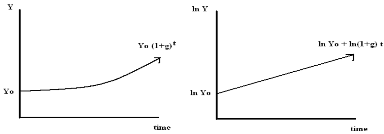
Recall that, with a constant growth rate $g$ and starting from time 0, output in time $t$ is:

\[Y_t = (1 + g)^t \cdot Y_0\]

Taking natural logs of both sides, we have:

\[\ln Y_t = \ln Y_0 + t \cdot \ln (1 + g)\]

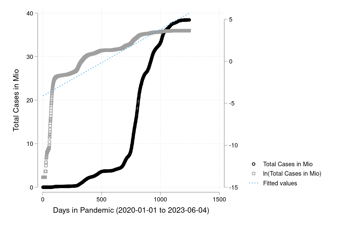
We see that log output is linear in time. Thus, if the growth rate is constant, a plot of log output against time will yield a straight line. Consequently, plotting log output against time is a quick way to eyeball whether growth rates have changed over time.

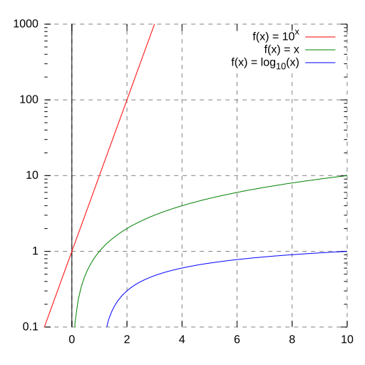
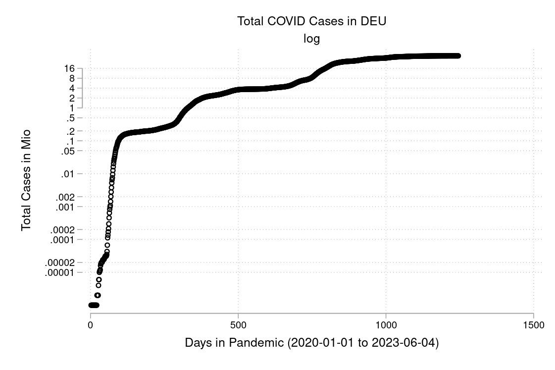
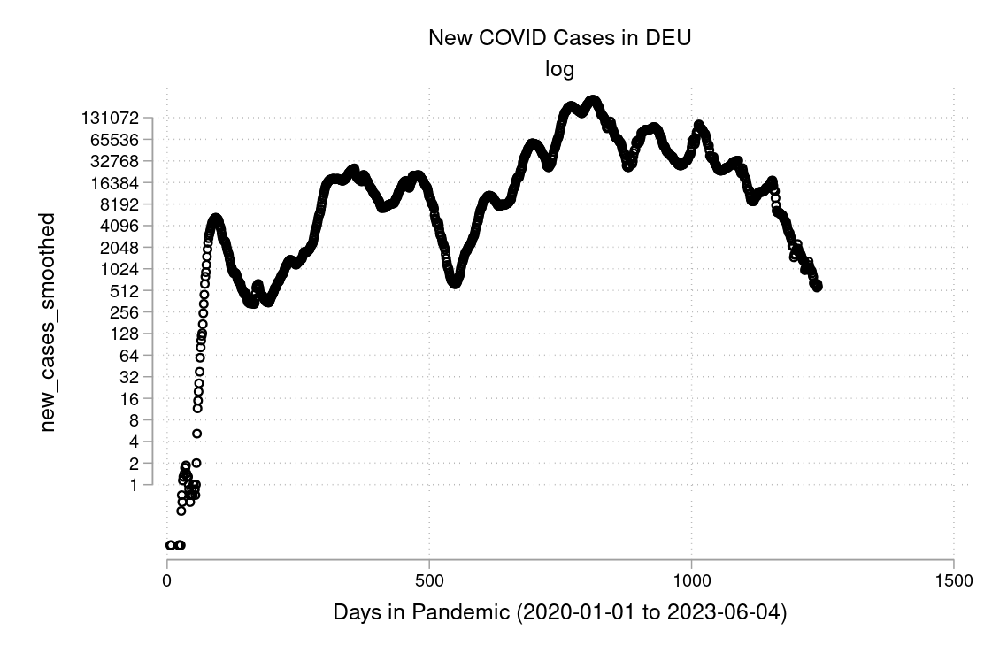
In Figure 9.1 and Figure 9.2 you see a semi-logarithmic plot that has one axis on a logarithmic scale and the other on a linear scale. It is useful for data with exponential relationships, where one variable covers a large range of values, or to zoom in and visualize that what seems to be a straight line in the beginning is, in fact, the slow start of a logarithmic curve that is about to spike, and changes are much bigger than thought initially.

Exercise 9.9 Investments over time

Describe the formulas to describe the growth process of an investment over time when time is discrete and when time is continuous.

Solution

The formula under discrete time is: \[ Y_t=Y_0\cdot (1+g)^t \] The formula under continuous time is: \[ Y_t=Y_0\cdot e^{gt} \]

Exercise 9.10 Exponential growth

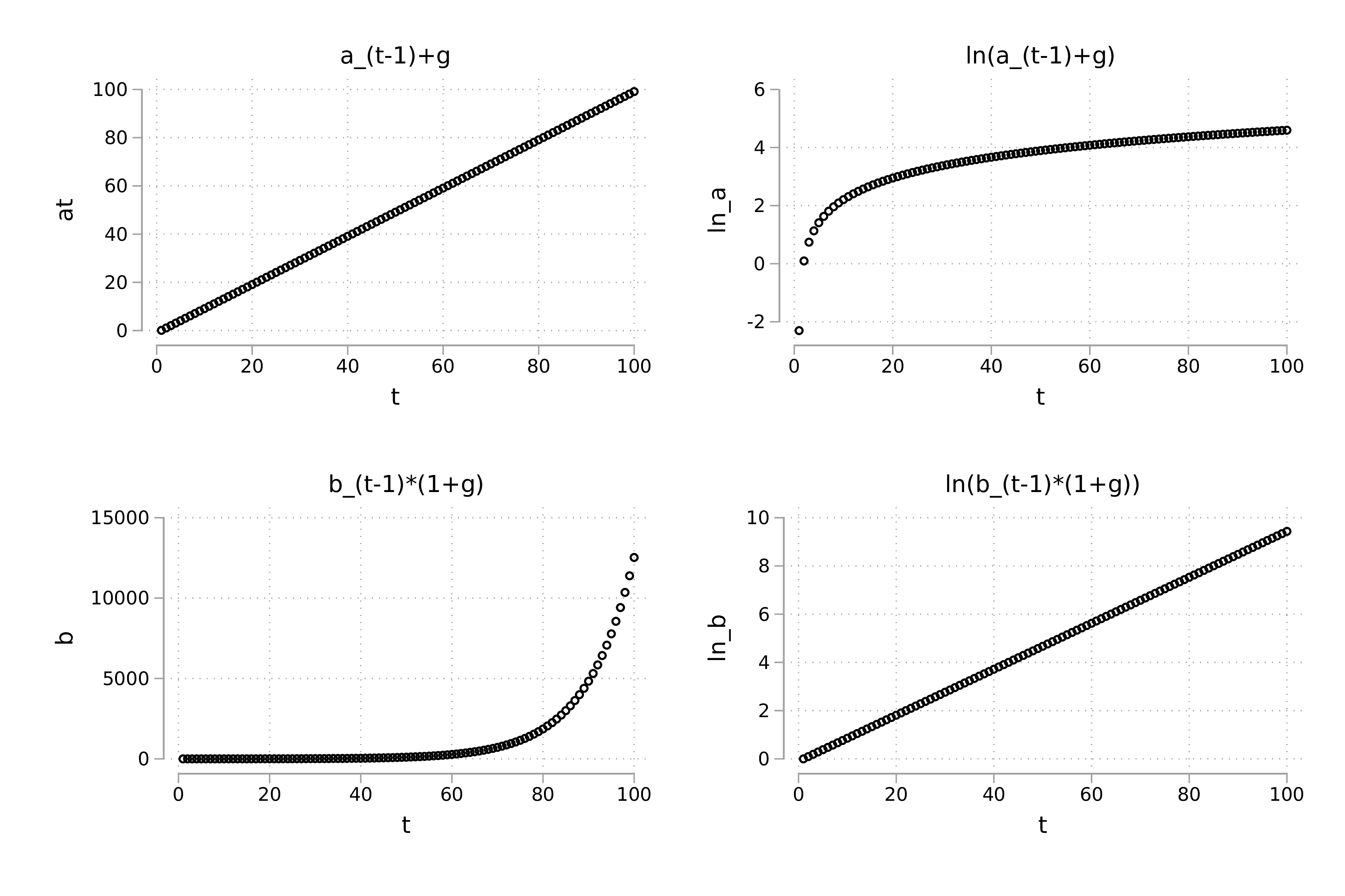
Sketch a timeline for each of the following series:

$a_t=a_{t-1}+g$
$\ln(a_t)$
$b_t=b_{t-1}\cdot (1+g)$
$\ln b_t$

Solution

Figure Figure 9.3 provides the solution.

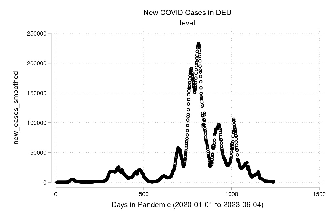
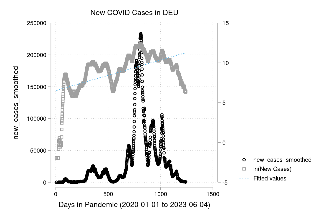
Exercise 9.11 COVID and how to plot it

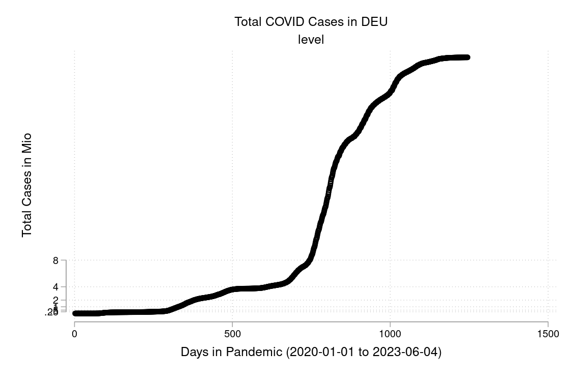
I downloaded the complete Our World in Data COVID-19 dataset from ourworldindata.org. I created some graphs which I will show you below in Figure 9.4 to Figure 9.9. Can you discuss the scaling and how to interpret them? What is your opinion on these graphs? Are some of them a bit misleading (at least if you don’t look twice)?