7  Conditional events

Learning outcomes

After successful completion of the module, students are able to:

  • Understand and use the terminology of probability.
  • Determine whether two events are mutually exclusive and whether two events are independent.
  • Calculate probabilities using the addition rules and multiplication rules.
  • Calculate with conditional probabilities using Bayes Theorem.
  • Construct and interpret venn and tree diagrams.
  • Apply their knowledge of probability theory to decision making in business.

When dealing with probabilities, especially conditional probabilities, relying on intuition and gut feeling often leads to poor decision-making. Our judgments are biased, and the choices we make are usually less rational than we may believe. Exercise 7.1 provides some evidence for my claim. Before I discuss how conditional probabilities can be considered in a rational decision making process, I repeat the essential basics of stochastics in Section 7.1

Exercise 7.1 Lisa is pregnant

The following question stems from a study carried out by Kahneman & Tversky (1972): Lisa is thirty-three and is pregnant for the first time. She is worried about birth defects such as Down syndrome. Her doctor tells her that she need not worry too much because there is only a 1 in 1,000 chance that a woman of her age will have a baby with Down syndrome. Nevertheless, Lisa remains anxious about this possibility and decides to obtain a test, known as the Triple Screen, that can detect Down syndrome. The test is moderately accurate: When a baby has Down syndrome, the test delivers a positive result 86 percent of the time. There is, however, a small ‘false positive’ rate: 5 percent of babies produce a positive result despite not having Down syndrome. Lisa takes the Triple Screen and obtains a positive result for Down syndrome.

Given this test result, what are the chances that her baby has Down syndrome?

  1. 0-20 percent chance
  2. 21-40 percent chance
  3. 41-60 percent chance
  4. 61-80 percent chance
  5. 81-100 percent chance

Think about the question and put your answer here:

https://pingo.coactum.de/ Code: 666528

At the beginning of the Inferential Statistics course at summer 2020, I also asked student this question. Here are the results of the 16 students who participated:

Option Frequency of answers Percentage
a) 3 19%
b) 2 13%
c) 2 13%
d) 3 19%
e) 6 38%

How did they reach their answers? Like most people, they decided that Lisa has a substantial chance of having a baby with Down syndrome. The test gets it right 86 percent of the time, right? That sounds rather reliable, doesn’t it? Well it does, but we should not rely on our feelings here and better do the math because the correct result would be that there is just a 1.7 percent chance of the baby having a Down syndrome.

Now, let us proof the result that there is just a 1.7 percent chance of the baby having a Down syndrome using Bayesian Arithmetic which is explained in the following videos:

Also, consider this interactive tool here: https://www.skobelevs.ie/BayesTheorem/

Let \(A\) be the event of the Baby has a Down syndrom and \(B\) the test is positive. Then, \[\begin{align*} P(A)&=0.001\\ P(B\mid A)&=0.86\\ P(B\mid \neg A)&=0.05\\ P(B)&=\frac{999\cdot 0.05}{1000}+\frac{1\cdot 0.86}{1000}=\frac{50.81}{1000}=0.05081\\ P(A\mid B)&={\frac {P(B\mid A)P(A)}{P(B)}}=\frac{0.86 \cdot 0.001}{0.05081}=0.016925802 \end{align*}\]

Kahneman, D., & Tversky, A. (1972). Subjective probability: A judgment of representativeness. Cognitive Psychology, 3(3), 430–454.

7.1 Terminology: \(P(A)\), \(P(A|B)\), \(\Omega\), \(\cap\), \(\neg\), …

Exercise 7.2  

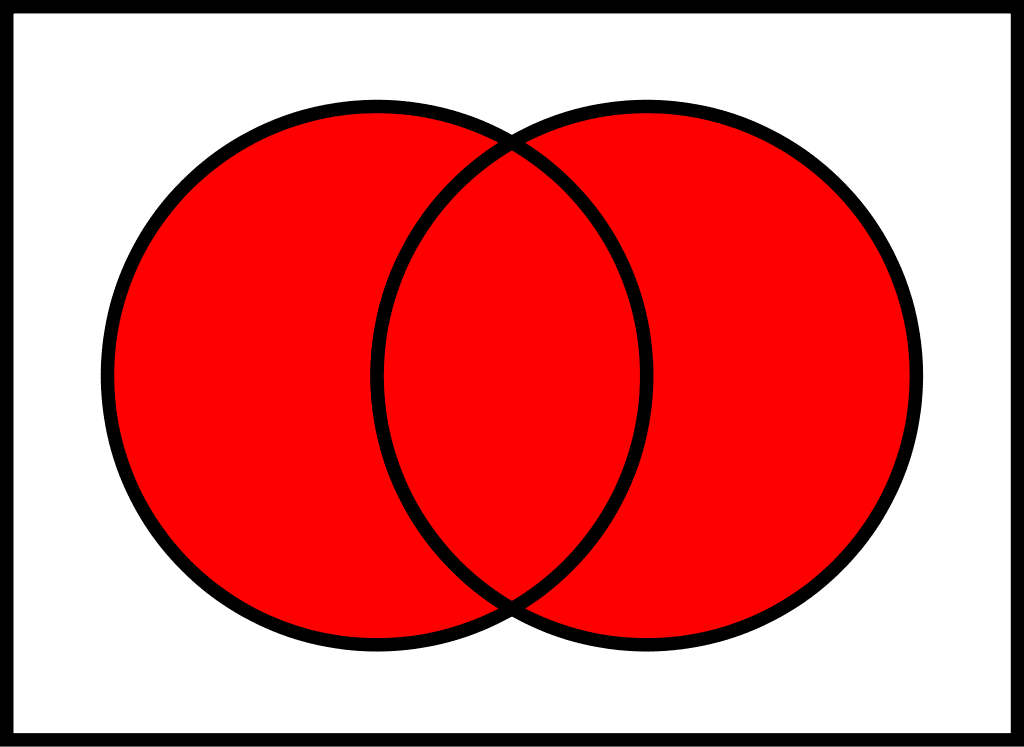
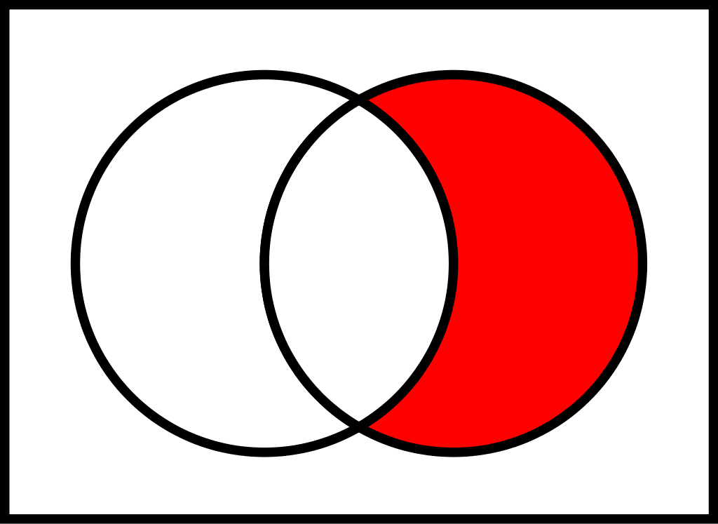
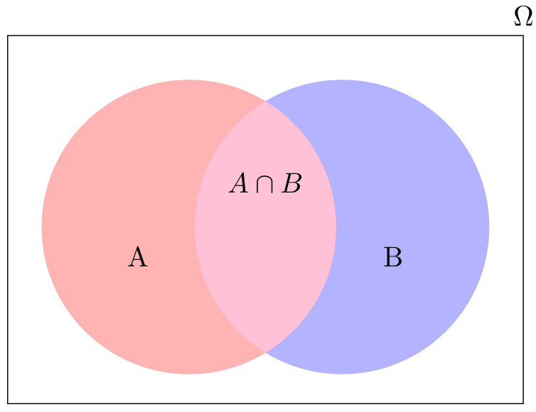
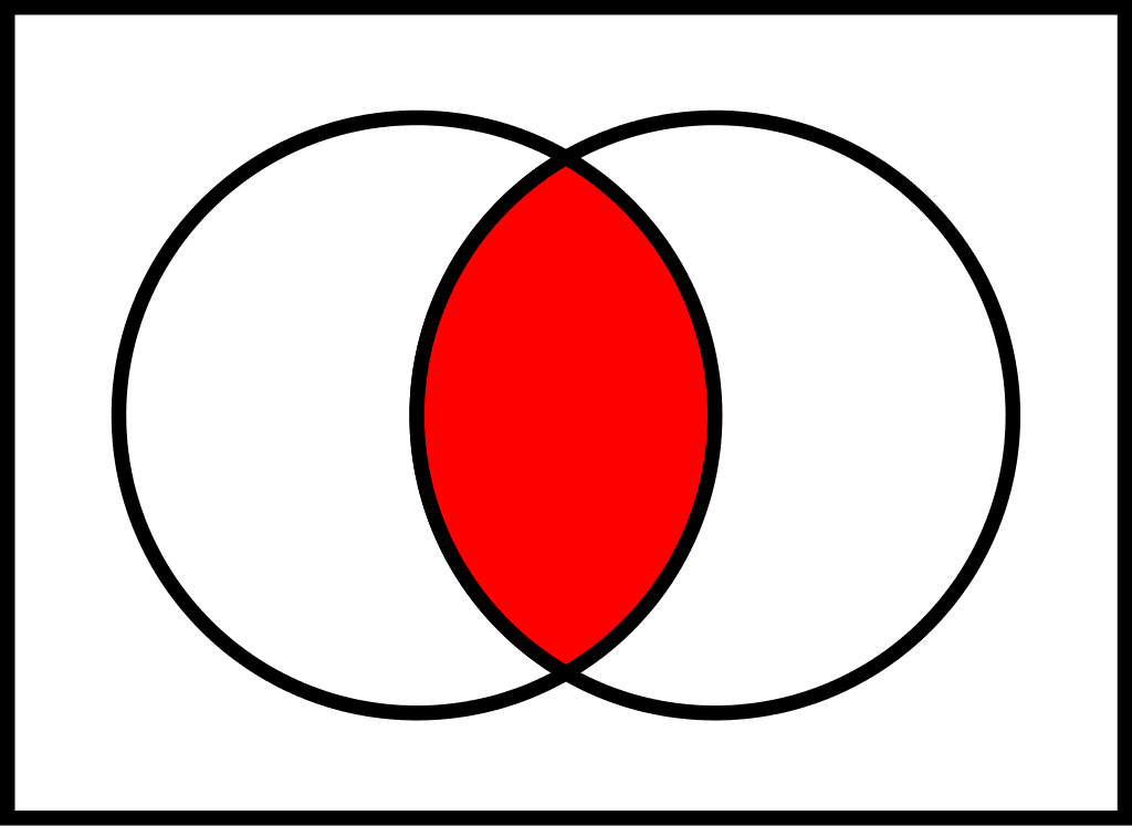
Figure 7.1: Set theory visualized
(a) Intersection: \(A \cap B\)
(b) Union: \(A \cup B\)
(c) Relative complement: \(\neg A \cup B\)

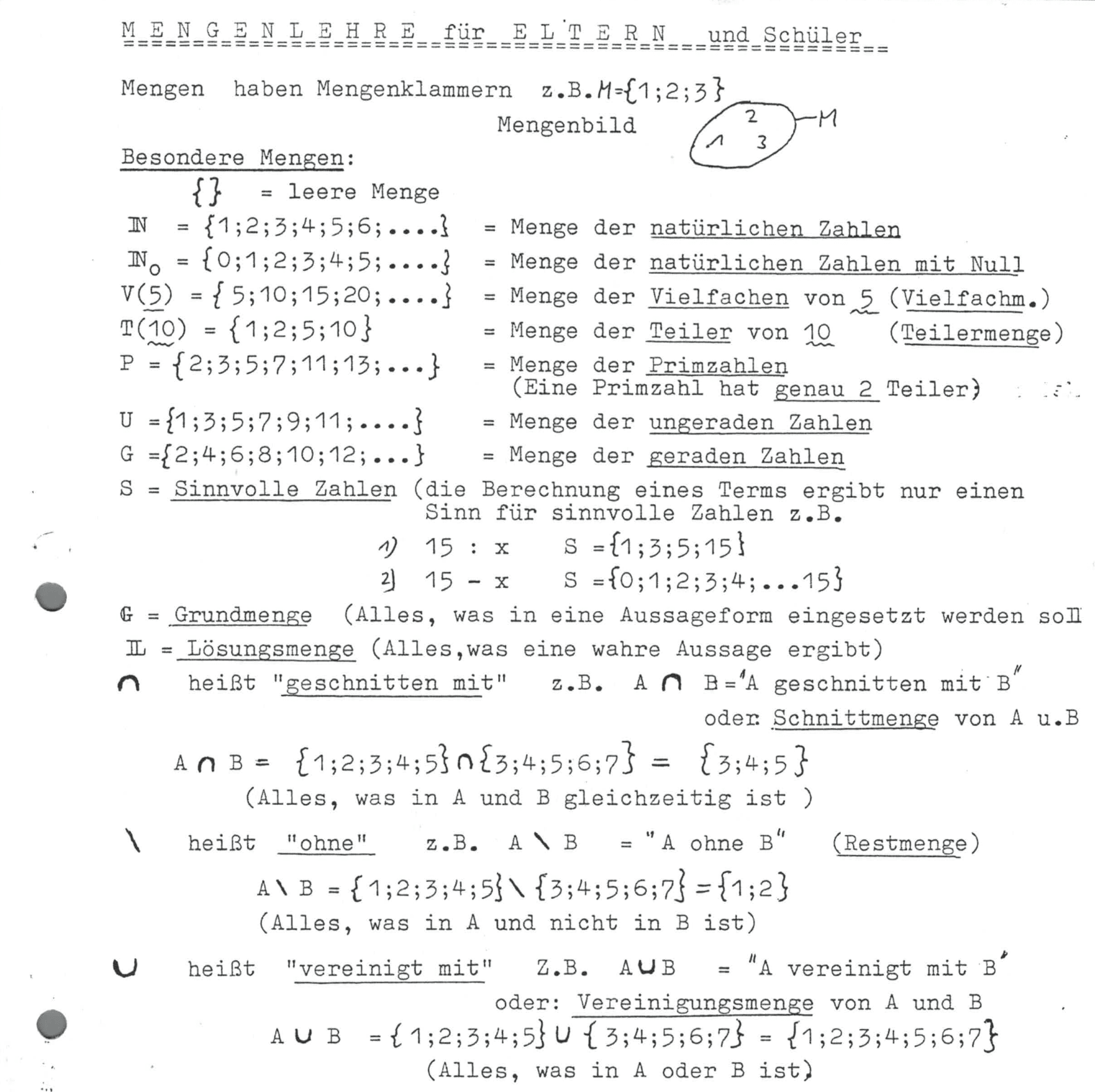
The next chapter will deal with stochastics, probabilities, and set theory. I guess you are somehow familiar with graphical visualization like shown in Figure 7.1. In Germany and most other countries, that is taught in school. When I moved to Cologne in 2020, I found the page shown in Figure 7.2 that I had received back then from my high school math teacher. It was September 1993 and I was a struggling fifth grader in my fourth week. Perhaps you’d like to share your experiences with stochastics?

Figure 7.2: Relative complement: \(\neg A \cup B\)

7.1.1 Sample space

A result of an experiment is called an outcome. An experiment is a planned operation carried out under controlled conditions. Flipping a fair coin twice is an example of an experiment. The sample space of an experiment is the set of all possible outcomes. The Greek letter \(\Omega\) is often used to denote the sample space. For example, if you flip a fair coin, \(\Omega = \{H, T\}\) where the outcomes heads and tails are denoted with \(H\) and \(T\), respectively.

Exercise 7.3 Sample space

Find the sample space for the following experiments:

  1. One coin is tossed.
  2. Two coins are tossed once.
  3. Two dices are tossed once.
  4. Picking two marbles, one at a time, from a bag that contains many blue, \(B\), and red marbles, \(R\).
  1. \(\Omega = \{head, tail\}\)
  2. \(\Omega = \{(head, head), (tail, tail),(head, tail),(tail, head)\}\)
  3. Overall, 36 different outcomes: \(\{ (1,1),(1,2),(1,3),(1,4),(1,5),(1,6),(2,1),(2,2),\dots,(6,6) \}\)
  4. \(\Omega = \{(B,B), (B,R), (R,B), (R,R)\}\).

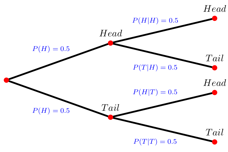
Overall, there are three ways to represent a sample space:

  1. to list the possible outcomes (see Exercise 7.3),
  2. to create a tree diagram (see Figure 7.3), or
  3. to create a Venn diagram (see Figure 7.4).
Figure 7.3: Tree diagramm
Figure 7.4: Venn diagramm

7.1.2 Probability

Probability is a measure that is associated with how certain we are of outcomes of a particular experiment or activity. The probability of an event \(A\), written \(P(A)\), is defined as \[ P(A)=\frac{\text{Number of outcomes favorable to the occurrence of } A}{\text{Total number of equally likely outcomes}}=\frac{n(A)}{n(\Omega)} \]

For example, A dice has 6 sides with 6 different numbers on it. In particular, the set of elements of a dice is \(M=\{1,2,3,4,5,6\}\). Thus, the probability to receive a 6 is 1/6 because we look for one wanted outcome in six possible outcomes.

Exercise 7.4 Probability

When a fair dice is thrown, what is the probability of getting

  1. the number 5,
  2. a number that is a multiple of 3,
  3. a number that is greater than 6,
  4. a positive number that is less than 7.

A fair dice is an unbiased dice where each of the six numbers is equally likely to turn up. The sample space is \(\Omega = \{1, 2, 3, 4, 5, 6\}\).

  1. Let A be the event of getting the number 5, \(A=\{5\}\). Then, \(P(A)=\frac{1}{6}\).
  2. Let \(B\) be the event of getting a multiple of 3, \(B=\{3, 6\}\). Then, \(P(B)=\frac{1}{3}\).
  3. Let \(C\) be the event of getting a number greater than 6, \(C=7,8,\dots\). Then, \(P(C)=0\) as there is no number greater than 6 in the sample space \(\Omega=\{1,2,3,4,5,6\}\). A probability of 0 means the event will never occur.
  4. Let D be the event of getting a number less than 7, \(D=\{1,2,3,4,5,6\}\). Then, \(P=1\) as the event will always occur.

7.1.2.1 The complement of an event (\(\neg-Event\))

The complement of event \(A\) is denoted with a \(\neg A\) or sometimes with a superscript `c’ like \(A^c\). It consists of all outcomes that are not in \(A\). Thus, it should be clear that \(P(A) + P(\neg A) = 1\). For example, let the sample space be \[\Omega = \{1, 2, 3, 4, 5, 6\}\] and let \[A = \{1, 2, 3, 4\}.\] Then, \[\neg A = \{5, 6\};\] \[P(A) = \frac{4}{6};\] \[P(\neg A) = \frac{2}{6};\] and \[P(A) + P(\neg A) = \frac{4}{6}+\frac{2}{6} = 1.\]

7.1.2.2 Independent events (AND-events)

Two events are independent when the outcome of the first event does not influence the outcome of the second event. For example, if you throw a dice and a coin, the number on the dice does not affect whether the result you get on the coin. More formally, two events are independent if the following are true: \[\begin{align*} P(A|B) &= P(A)\\ P(B|A) &= P(B)\\ P(A \cap B) &= P(A)P(B) \end{align*}\]

To calculate the probability of two independent events (\(X\) and \(Y\)) happen, the probability of the first event, \(P(X)\), has to be multiplied with the probability of the second event, \(P(Y)\): \[ P(X \text{ and } Y)=P(X \cap Y)=P(X)\cdot P(Y),\] where \(\cap\) stands for “and”.

For example, let \(A\) and \(B\) be \(\{1, 2, 3, 4, 5\}\) and \(\{4, 5, 6, 7, 8\}\), respectively. Then \(A \cap B = \{4, 5\}\).

Exercise 7.5 Three dices

Suppose you have three dice. Calculate the probability of getting three times a 4.

The probability of getting a \(4\) on one dice is 1/6. The probability of getting three \(4\) is: \[ P(4 \cap 4 \cap 4) = \frac{1}{6}\cdot \frac{1}{6}\cdot \frac{1}{6}= \frac{1}{216} \]

7.1.2.3 Dependent events (\(|\)-Events)

Events are dependent when one event affects the outcome of the other. If \(A\) and \(B\) are dependent events then the probability of both occurring is the product of the probability of \(A\) and the probability of \(A\) after \(B\) has occurred: \[ P(A \cap B)=P(A)\cdot P(B|A) \] where \(|A\) stands for “after A has occurred”, or “given A has occurred”. In other words, \(P(B|A)\) is the probability of \(B\) given \(A\).

Of course, the equation above can also be written as \[ \Leftrightarrow P(B|A)=\frac{P(A \cap B)}{P(A)}\cdot. \]

For example, suppose we toss a fair, six-sided die. The sample space is \(\Omega = \{1, 2, 3, 4, 5, 6\}\). Let \(A\) be 2 and 3 and let \(B\) be even (2, 4, 6). To calculate \(P(A|B)\), we count the number of outcomes 2 or 3 in the sample space \(B = \{2, 4, 6\}\). Then we divide that by the number of outcomes \(B\) (rather than \(\Omega\)).

We get the same result by using the formula. Remember that \(\Omega\) has six outcomes. \[P(A\mid B)=\frac{P(B\cap A)}{P(B)} = \frac{\frac{\text{number of outcomes that are 2 or 3 AND even}}{6}}{\frac{\text{number of outcomes that are even}}{6}}=\frac{\frac{1}{6}}{\frac{3}{6}}=\frac{1}{3} \]

Exercise 7.6 Purse

A purse contains four € 5 bills, five € 10 bills and three € 20 bills. Two bills are selected randomly without the first selection being replaced. Find the probability that two € 5 bills are selected.

There are four € 5 bills. There are a total of twelve bills. The probability to select at first a € 5 bill then is \(P(\text{€} 5) = \frac{4}{12}\). As the the result of the first draw affects the probability of the second draw, we have to consider that there are only three € 5 bills left and there are a total of eleven bills left. Thus, \[ P(\text{€} 5 | \text{€} 5)=\frac{3}{11} \] and \[ P(\text{€} 5 \cap \text{€} 5) = P(\text{€} 5) \cdot P(\text{€} 5 | \text{€} 5) = \frac{4}{12} \cdot \frac{3}{11}=\frac{1}{11}. \] The probability of drawing a € 5 bill and then another € 5 bill is \(\frac{1}{11}\).

7.2 Bayes’ Theorem

The conditional probability of A given B is written \(P(A|B)\). \(P(A|B)\) is the probability that event A will occur given that the event B has already occurred. A conditional reduces the sample space. We calculate the probability of A from the reduced sample space B. The formula to calculate \(P(A|B)\) is \[ P(A|B) = \frac{P\left(A\cap B\right)}{P\left(B\right)}\] where \(P(B)\) is greater than zero. This formula is also known as Bayes’ Theorem, which is a simple mathematical formula used for calculating conditional probabilities, states that \[ P(A)P(B|A)=P(B)P(A|B) \] This is true since \(P(A \cap B)=P(B \cap A)\) and due to the fact that \(P(A\cap B)=P(B\mid A)P(A)\), we can write Bayes’ Theorem as \[P(A\mid B)={\frac {P(B\mid A)P(A)}{P(B)}}.\] The box below summarizes the important facts w.r.t. Bayes’ Theorem.

Bayes’ Theorem

The theorem states that \[P(A\mid B)={\frac {P(B\mid A)P(A)}{P(B)}} \] if \(P(B)\neq 0\) and \(A\) and \(B\) are events. It simply uses the following logical facts: \[P(B\cap A)=P(A\cap B),\] \[P(A\mid B)=\frac {P(A\cap B)}{P(B)}, \text{ and}\] \[P(B\mid A)=\frac {P(A\cap B)}{P(A)},\] or, to put it in one line: \[ P(A\cap B)= P(B\cap A)=P(A\mid B)P(B)=P(B\mid A)P(A). \] Sometimes, it is helpful to re-write the Theorem as follows: \[P(A)=P(A|B)P(B)+P(A|\neg B)P(\neg B), \text{ and}\] \[P(B)=P(B|A)P(A)+P(B|\neg A)P(\neg A),\]

For a deeper understanding of Bayes theorem, I recommend watching the following videos:

Moreover, this interactive tool can be helpful.
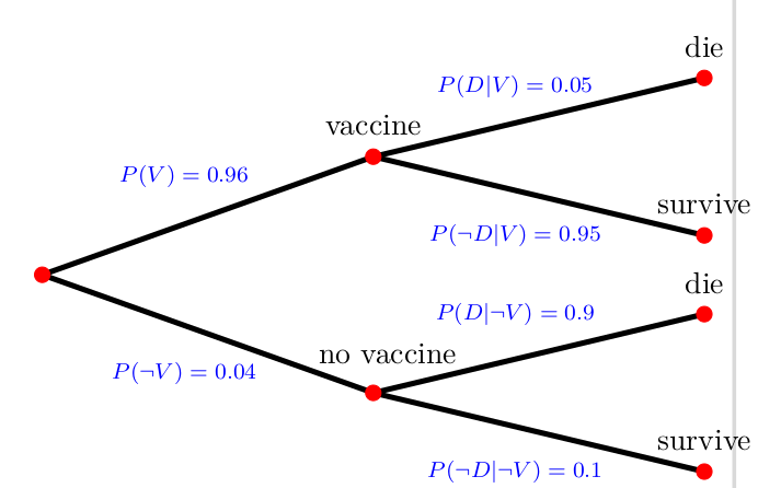
Exercise 7.7 To be vaccinated or not to be

Figure 7.5: Tree diagramm (Exercise 7.7)

The tree diagram in Figure 7.5 shows probabilities of people to have a vaccine for some disease. Moreover, it shows the conditional probabilities of people to die given the fact they were vaccinated or not. \(D\) denotes the event of die and \(\neg D\) denotes not die, i.e., survive; \(V\) denotes the event of vaccinated and \(\neg V\) not vaccinated.

  1. Calculate the overall probability to die, \(P(D)\)
  2. Calculate the probability that a person that has died was vaccinated, \(P(V|D)\).

Disclaimer: The case presented here is fictitious. The data given here are purely fictitious and serve only to practice the method.

  1. \[\begin{align*} P(D)&=P(V)\cdot P(D|V)+(P(\neg V)\cdot P(D|\neg V))\\ &= .96\cdot .05 + .04 \cdot .09\\ &= 0.048 + 0.036 \\&= 0.084 \end{align*}\]
  2. \[\begin{align*} P(V \mid D)={\frac {P(D\mid V)P(V)}{P(D)}}= \frac{.05\cdot .96}{.084}\approx .5714285 \end{align*}\]

Exercise 7.8 To die or not to die

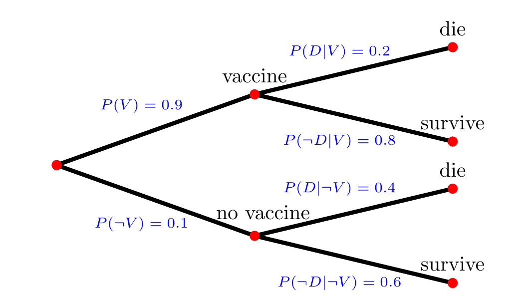
You read on Facebook that in the year 2021 about over 80% of people that died were vaccinated. You are shocked by this high probability that a dead person was vaccinated, \(P(V|D)\). You decide to check this fact. Reading the study to which the Facebook post is referring, you find out that the study only refers to people above the age of 90. Moreover, you find the following Tree Diargram. It allows checking the fact as it describes the vaccination rates and the conditional probabilities of people to die given the fact they were vaccinated or not. In particular, \(D\) denotes the event of die and \(\neg D\) denotes not die, i.e., survive; \(V\) denotes the event of vaccinated and \(\neg V\) not vaccinated.

Figure 7.6: Tree diagramm (Exercise 7.8)
  1. Calculate the overall probability to die, \(P(D)\)
  2. Calculate the probability that a person that has died was vaccinated, \(P(V|D)\).
  3. Your calculations shows that the fact used in the statement on Facebook is indeed true. Discuss whether this number should have an impact to get vaccinated or not.

Disclaimer: The case presented here is fictitious. The data given here are purely fictitious and serve only to practice the method.

  1. \[P(D) = 0.9\cdot0.2+0.1\cdot0.4=0.22\]
  2. \[P(V\mid D)=\frac P(D\mid V)P(V)P(D)=\frac0.2\cdot 0.90.22=\frac0.0360.22\approx0.8181\] % \[P(\neg V\mid D)=\frac P(D\mid \neg V)P(\neg V)P(D)=\frac0.4\cdot 0.40.028=\frac0.020.028\approx0.71428\]

Exercise 7.9 Corona false positive

Suppose that Corona infects one out of every 1000 people in a population and that the test for it comes back positive in 99% of all cases if a person has Corona. Moreover, the test also produces some false positive, that is about 2% of uninfected patients also tested positive.

Now, assume you are tested positive and you want to know the chances of having the disease. Then, we have two events to work with:

A: you have Corona

B: your test indicates that you have Corona

and we know that \[\begin{align*} P(A)&=.001 \qquad \rightarrow \text{one out of 1000 has Corona}\\ P(B|A)&=.99 \qquad \rightarrow \text{probability of a positive test, given infection}\\ P(B|\neg A)&=.02 \qquad \rightarrow \text{probability of a false positive, given no infection} \end{align*}\]

As you don’t like to go into quarantine, you are interested in the probability of having the disease given a positive test, that is \(P(A|B)\)?

Disclaimer: The case presented here is fictitious. The data given here are purely fictitious and serve only to practice the method.

In order to come to an answer, lets draw a table of the probabilities that may be of interest:

A \(\neg A\) \(\sum\)
B \(P(A\cap B)\) \(P(\neg A \cap B)\) \(P(B)\)
\(\neg B\) \(P(A \cap \neg B)\) \(P(\neg A \cap \neg B)\) \(P(\neg B)\)
\(P(A)\) \(P(\neg A)\) 1

Please note, the symbol \(\neg\) simply abbreviates “NOT” and the symbol \(\cap\) stands for “AND”. The probability of you having both the disease and a positive test, \(P(A \cap B)\), is easy to calculate: \[\underbrace{P(A \cap B)= P(B|A)P(A)}_{\text{a.k.a. multiplication rule}}=.99\cdot .001=.00099\] Also, it is straight forward to calculate the probability of having both, no infection and a positive test: \[ P(\neg A \cap B)= P(B|\neg A)P(\neg A)=.02\cdot .999 = .01998 \] Knowing that, it is clear that the overall probability of being diagnosed with Corona is \[P(B)=.00099+.0199=.02097\] That means, out of 1000 people about 21 are on average diagnosed with Corona while only one person actually is infected with Corona. Thus, your probability of having Corona once your test came out to be positive, \(P(A|B)\), is approximately \[P(A|B) \approx \frac{1}{21}=0,047619048\] and more precisely \[ P(A|B)=\frac{P(A\cap B)}{P(B)}=\frac{.00099}{.02097}=0,0472103. \]

In other words, with a probability of more than 95%, you may go into quarantine without infection: \[ P(\neg A|B)=\frac{P(\neg A\cap B)}{P(B)}=\frac{.01998}{.02097}=0,9527897\quad (=1-P(A|B)) \]

Given the accuracy of the test, this number appears to be rather high to many people. The high test accuracy of 99% and the rather low number of 2% false positives, however, is misleading. This is sometimes called the . The source of the fact that many people think \(P(A|B)\) is much lower is that they don’t consider the impact of the low probability of having the disease, \(P(A)\), on \(P(A|B)\), \(P(B|A)\), and \(P(B|\neg A)\) respectively (also, see the ). Moreover, many people don’t understand the false positive rate correctly.

To summarize, we know

A ¬A \(\sum\)
B .00099 .01998 .02097
¬B P(A ¬B) P(¬A ¬B) P(¬B)
.001 P(¬A) 1

The four remaining unknowns can be calculated by subtracting in the columns and adding across the crows, so that the final table is:

A ¬A \(\sum\)
B .00099 .01998 .02097
¬B .00001 .97902 .97903
.001 .999 1