26 Strategic trade policy

26.1 Gains from trade

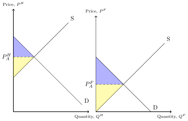
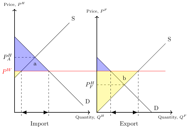
Figure 26.1 and Figure 26.2 contain domestic supply and demand curves. In autarky with no possibilities to trade, supply and demand must meet. Under free trade and a given world market price, $P^W$, countries can trade with each other. This has implications for the producer surplus (yellow area) and the consumer surplus (blue area), as shown in the figures. The area of the triangles a and b as denoted in Figure 26.2 represents the welfare gain from free trade that can be achieved given the world market price, $P^W$.

Figure 26.2: Two countries that trade with each other

26.2 Tariffs in small open economies

Figure 26.3 can teach us a lot about the impact of a tariff $t$ on trade and welfare. A tariff raises the domestic price of imported goods. If we assume that the imposition or change of a country’s tariff has no effect on the world price, we consider what is called a small open economy, which is so small that the country’s consumption and production decisions do not affect the world price. In other words, the country takes the world price for granted because its import demand does not change the world price.

In autarky, the economy represented in Figure 26.3 would consume 5 units at price $P^A$, and total welfare would be represented by areas $a+b_2+b_1$. Under free trade without tariffs, the country imports 8 units and consumes 9 units at the price of $P^W$. The consumer surplus corresponds to areas $a+b_2+d_1+c+d_2$ and the producer surplus corresponds to area $b_1$. After the introduction of tariff $t$, the consumer surplus is equal to area $a$ and the producer surplus is equal to area $b_1+b_2$. Thus, consumer surplus has decreased while producer surplus has increased. The area $c$ is equal to the government’s revenue. It represents the portion of the consumer welfare loss that is transferred to the government. Overall, welfare has decreased. The welfare loss is equal to the areas of the two triangles $d_1$ and $d_2$. These triangles represent what is called the deadweight loss due to the tariff.
Specifically, triangle $d_1$ represents the reduction in imports that is replaced by domestic production, and triangle $d_2$ represents the loss in consumption due to a reduction in imports and a reduction in domestic consumption.

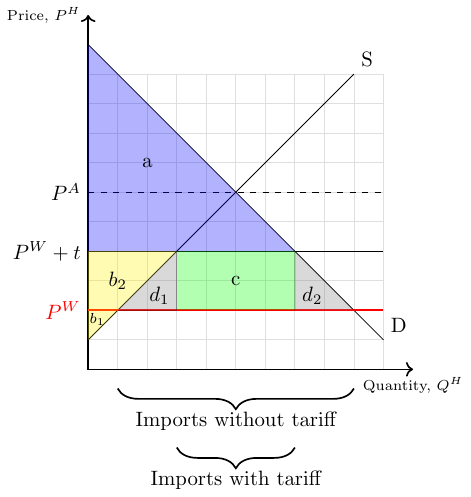
Figure 26.3: Tariff in a small open economy

The implications of a tariff in a small economy

While a tariff protects domestic producers and increases their surplus, it reduces the surplus of consumers and leads to a deadweight loss of revenue. Overall, a tariff leads to a reduction in a country’s welfare.

26.3 Quotas in small open economies

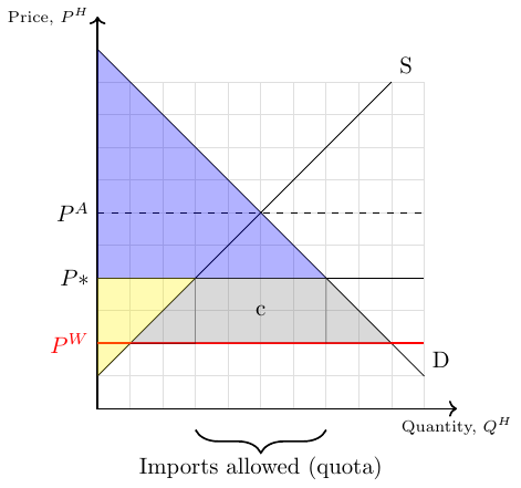
A trade restriction that sets a physical limit on the quantity of a good to be imported is called an import quota. It gives government officials more power and control than a tariff because they can strictly limit the quantity of goods traded and have the administrative authority to grant (or sell) import licenses to certain foreign exporters.

Figure 26.4 shows the impact of an import quota that allows an import quantity of 4 units. In this scenario, 7 units are consumed, four of which are imported. The price at which all seven units are consumed is $P*$. This is somewhat surprising because the world price $P^W$ is less than $P^*$. The reason is that all firms that are allowed to sell their products do so at the highest possible price, that is, $P^*$. As above, the blue area is the consumer surplus and the yellow area is the producer surplus. The gray area is the loss in value due to the import rate. The rectangle $c$ is only part of this loss, since we assume that the government does not sell the licenses to the best bidding exporting firm

Figure 26.4: Tariff in a small open economy

26.4 Tariffs in large open economies

So far, we have assumed that the country of interest is small and takes the world market price as given. However, large countries’ demand for imported goods can have an impact on world prices. If this is the case, we can show that a tariff can actually improve a country’s welfare. Figure 26.5 illustrates the effects of a tariff on welfare, prices, and trade. In particular, we show the impact of a small tariff of 6 euros per bicycle.

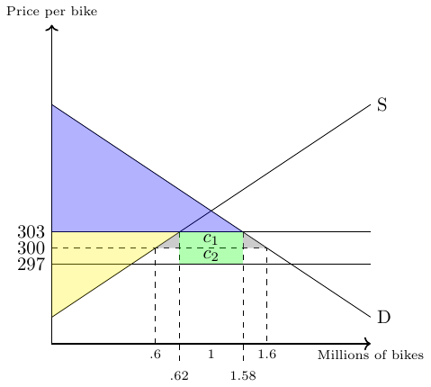
Figure 26.5: The effect of a tariff in a large country

Under free trade, the market for bicycle imports is cleared at a price of €300 and the country imports one million bicycles.

Now, if a tariff of 6€ per bicycle is imposed, the tariff drives a wedge between the price foreign exporters receive and the price domestic buyers of imports pay. That is, it becomes more expensive for domestic buyers to purchase imported bicycles. This, in turn, leads to an immediate drop in domestic demand for bicycles and pushes the world market price for bicycles to €297 Given the new world market price for bicycles, the domestic price for imported bicycles is €303 (297+6).

The consumer surplus is now represented by the blue area and the producer surplus by the yellow area. The green area represents the tariff revenue collected by the government. The two gray triangles, in turn, show the tariff-related deadweight losses. Compared to the free trade scenario, the country gains rectangle $c_2$. If the revenue in this area is greater than the deadweight loss, the country has improved its overall welfare by imposing a tariff.

Let us calculate whether this is the case here:

Area $c_2$: \[ (1.58 \text{ million bikes} - 0.62 \text{ million bikes})\cdot (\text{€} 300-\text{€} 297)=\text{€} 2.88 \text{ million} \]
Deadweight loss: \[\begin{align} \underbrace{\frac{(0.62 \text{ mio b.}-0.6 \text{ mio b.})\cdot (\text{€} 303 - \text{€} 300)}{2}}_{\text{left triangle}} + \\ \underbrace{\frac{(1.6 \text{ mio b.}-1.58 \text{ mio b.})\cdot (\text{€} 303 - \text{€} 300)}{2}}_{\text{right triangle}}\\ =\text{€} 0.06 \text{ million} \end{align}\]
Indeed, the net gain is €2.82 million. Thus, a small tariff can increase the welfare of a country.

26.5 Other nontariff trade barriers

In addition to tariffs, there are a variety of other trade barriers. These so-called non-tariff barriers (NTBs) include quotas, export subsidies, domestic production subsidies, government buy-at-home policies, and product standards. Here is a more complete list:

Import quotas
Voluntary export restraints
Antidumping laws
Exchange-rate controls
Countervailing duties
Government subsidies
Licensing, labeling and packaging restrictions
Quality controls and technical standards
Domestic-content laws
Political rhetoric
Embargoes and sanctions
Most/least-favored nation status

For example, product standards are much more important than you might think. For example, no car from the United States can be sold in the European Union without modifications because our safety standards are different. Another example is the CE marking (see below). Harmonization of product standards is usually an important issue in trade agreements.

CE Marking

The CE marking shown in Figure 26.6 is one example for a non tariff trade barrier. It is not an abbreviation for China Export, as many believe. While CE is sometimes indicated as an abbreviation of Conformite Europeenne (French for European Conformity), it is not defined as such in the relevant legislation. The mark indicates that the product may be sold freely in any part of the European Economic Area, irrespective of its country of origin. The CE marking is a declaration by the manufacturer (not by some authority!) that the product complies with EU standards for health, safety and environmental protection for products sold within the European Economic Area (EEA). Thus, it is not a quality indicator or a certification mark and may also be found on products sold outside the EEA. You may also know the _FCC Declaration of Conformity} which is used for selling certain electronic devices in the United States.

Exercise 26.1 Tariff (Solution 26.1)

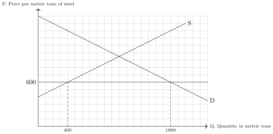
Referring to Figure 26.7, the government of a large country needs your help to decide whether the introduction of a tariff of $100 per metric ton of on steel is a good idea, or not. At the current world market price of $p^W=$ 600$, the country imports 14 millions metric tons of steel. The government expects that a tariff of $100 per ton of steel would decrease the world market price of steel for $1.

Calculate how much the overall welfare gain (or loss) of the country would be in case the government decides to introduce a tariff of $ 100 per ton of steel. Assume thereby that the supply curve is given by \[ P^s=400+\frac{1}{2}Q^s \] and the demand curve is given by \[ P^d=1500-\frac{1}{2}Q^d. \] These curves are also shown in the figure below.
What would be the tariff so high that it makes an import of steel prohibitively expensive.
What would be the world market price so low that it makes any domestic production unprofitable.
What would be the world market price so high that the country exports steel.

Solution 26.1. Tariff (Exercise 26.1)

By analogy with Figure 26.5, here we should compare the two gray triangles with area $c_2$.

The price per metric ton of steel from foreign suppliers will be $699 because government will charge $100 on each ton of steel which is now worth $599 on world markets. As $699 is still below the autarky price of $950, domestic suppliers will set prices to be equal to $699. Thus,

\[\begin{align*} 699&=400+\frac{1}{2}Q^s \Leftrightarrow Q^s=598\\ 699&=1500-\frac{1}{2}Q^d \Leftrightarrow Q^d=1602\\ 1602-598 &=1004 \end{align*}\] That means, at a price of $699 domestic supply is 598 and domestic demand is 1602 tons of steel. 1004 tons will be imported.

To calculate the welfare loss (the two triangles), we can calculate the left triangle only and double it (please note that this is only possible if both triangles really have the same size which is only the case if both supply and demand curves have the same slope in absolute terms!): \[\begin{align*} & \overbrace{\left(\underbrace{(598-400)}_{\text{loss in quantity}}\cdot \underbrace{\frac{1}{2}}_{\text{to get the triangle}}\cdot \underbrace{(699-600)}_{\text{increase in price}}\right)}^{\text{left triangle}} \cdot \overbrace{2}^{\text{right triangle is of same size}}\\ &=9801\cdot 2\\ &=19602 \end{align*}\] The welfare gain (the new square that is due to the change in world market price, a.k.a. $c_2$) is \[ 1004 \text{tons} \cdot 1 \left[ \frac{\text{\$}}{\text{tons}} \right] = 1004 \text{\$}. \] Thus, overall welfare gain is \[ 1004-19602=-18598. \] That means, the welfare loss exceeds the welfare gain by $ 18598.

\[\begin{align*} 400+\frac{1}{2}Q&=1500-\frac{1}{2}Q\\ \Leftrightarrow Q&=1100\\ P^s&=400+\frac{1}{2}\cdot 1100\\ P^s&=950 \end{align*}\] At a price above $950, no steel would be imported. Thus, a tariff must be so high that the price of foreign steel within the country exceeds $950, that is, $P^W+t>950$. Assuming that the world market price would have a lower bound of $599, that is, any tariff above $100 would not decrease the world market price any further, a tariff of $351 (950-599=351) would make imported steel prohibitively expensive.

Below a price of $400 any domestic production would be unprofitable because the supply curve tells us that no domestic producer would be able to supply anything at and below the price of $400. To proof that just set $Q^s=0$ in the function of the supply curve and you get $P^s=400$.
At a world market price above $950, it would be profitable to export steel because domestic supply exceeds domestic demand and the world market price is higher than the production costs.