12 Elasticity
Required reading: Shapiro et al. (2022, ch. 5)
Learning objectives:
Students will be able to:
- Explain the concept of price elasticity of demand and how to calculate it.
- Describe what it means for demand to be price inelastic, unit price elastic, price elastic, perfectly price inelastic, and perfectly price elastic.
- Explain how and why the value of price elasticity of demand changes along a linear demand curve.
- Understand the relationship between total revenue and price elasticity of demand.
12.1 How to measure an elasticity
Elasticity is the measurement of the percentage change of one economic variable in response to a change in another. Here, elasticity refers to the degree to which individuals, consumers, or producers change their demand or the amount supplied in response to price or income changes. Elasticity is a normalized measure, meaning the units of measurement of the variables (€, cent, kg, g) do not play a role, enabling comparisons of how different goods react to price changes, for example.
The price elasticity of demand (PED) is computed as the percentage change in the quantity demanded divided by the percentage change in price:
\[ \text{PED} = \frac{\text{Percentage change in quantity demanded}}{\text{Percentage change in price}} = \frac{\frac{q_{t=\text{today}} - q_{t=\text{yesterday}}}{q_{t=\text{yesterday}}}}{\frac{p_{t=\text{today}} - p_{t=\text{yesterday}}}{p_{t=\text{yesterday}}}} \]
12.2 Midpoint method
The midpoint formula computes percentage changes by dividing the change by the average value (i.e., the midpoint) of the initial and final value. It is independent of the direction of change and hence is preferable to the basic method. For example, when a change in price from P_1 to P_2 comes along with a change in demand from Q_1 to Q_2, the formula can be written like this:
\[ \text{Price Elasticity of Demand (PED)} = \frac{\frac{Q_2 - Q_1}{\left(\frac{(Q_2 + Q_1)}{2}\right)}}{\frac{(P_2 - P_1)}{\left(\frac{(P_2 + P_1)}{2}\right)}} = \frac{\triangle Q / \bar{Q}}{\triangle P / \bar{P}} \]
Notice that the formula can be simplified by using the \(\triangle\) symbol to represent a change in values, and using a bar over the quantities to indicate the average of the two values.
12.3 Point elasticity
More generally, we can use differential calculus to get the the elasticity of two variables, x and y: \[ \epsilon_{y,x} = \frac{d Q }{d P}\cdot \frac{P}{Q} \]
12.4 Elasticity and demand
Price elasticity of demand (PED) has various classifications that help us understand how quantity demanded responds to price changes. It is termed perfectly elastic when \(|PED| \rightarrow \infty\), indicating that quantity responds infinitely to even the smallest price change. Conversely, it is labeled perfectly inelastic when \(PED = 0\), signifying that quantity does not respond at all to price changes.
In less extreme cases, we refer to price inelastic demand when \(0 < |PED| < 1\), meaning that quantity demanded does not respond significantly to changes in price. On the other hand, price elastic demand occurs when \(|PED| > 1\), indicating a strong responsive relationship between quantity demanded and price.
Understanding PED is crucial as it measures the sensitivity of quantity demanded to price changes and is closely related to the slope of the demand curve. However, it is important to note that the slope alone does not provide the complete picture of PED.
Determinants of PED: Several factors influence the price elasticity of demand. The availability of close substitutes plays a significant role, as does the classification of goods into necessities versus luxuries. Additionally, the time horizon can impact elasticity.
Price elasticity of a linear demand curve:
When examining the price elasticity of a linear demand curve, it is essential to recognize that while the slope remains constant, elasticity does not! Demand is typically inelastic at points with low prices and high quantities, whereas it becomes elastic at points with high prices and low quantities. This is demonstrated in Figure 12.1 and Figure 12.2.
Moreover, total revenue varies at each point along the demand curve. Demand curves with a constant price elasticity are referred to as iso-elastic. An iso-elastic demand curve is shown in panel (c) of Figure 12.1.
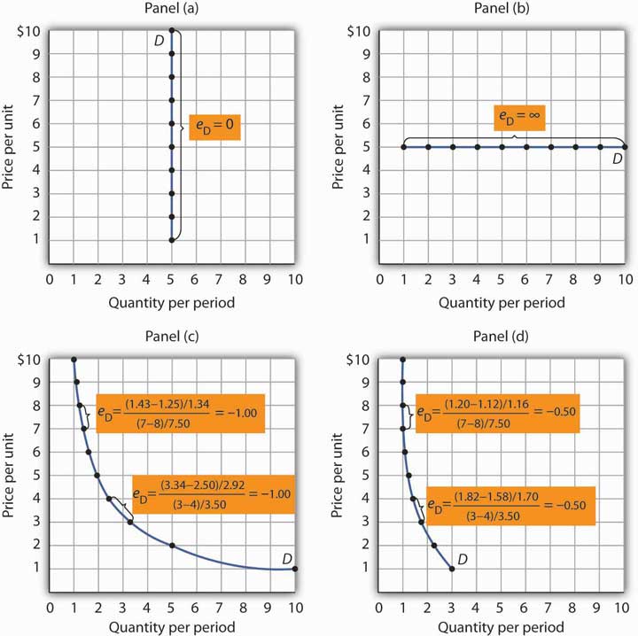
Source: Anon (2020, p. 154)
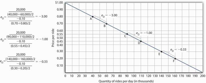
Source: Anon (2020, p. 148)