35 The specific factor model
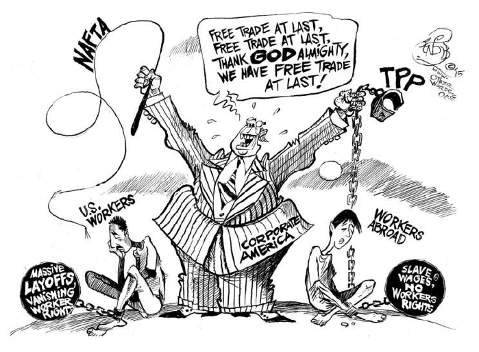
Source: otherwords.org
From the Ricardian model, we know that trade is a positive-sum game. If free trade is beneficial to a country, as Ricardo predicts, why isn’t everyone happy with free trade? In democratic societies, policymakers sometimes adopt protectionist trade policies because of pressure from interest groups and public demand. The discrepancy between the promises and potential benefits of trade on the one hand and the negative consequences of free trade for many groups on the other is illustrated in Figure 35.1. The models so far do not give us a way to see which groups actually suffer from free trade, and thus we have no clue why there are incentives for interest groups to oppose free trade. Are anti-free trade policy preferences the result of ignorance, general worldviews, political ideology, environmental attitudes, social trust, or other factors? Well, these things may play a role, but there are also economic factors, that is, the self-interest of individuals and groups within an economy, that can account for anti-free trade attitudes. In the following sections, we will discuss a theory that shows that while free trade benefits countries as a whole, not everyone within a country benefits equally. Some benefit more than others, and some are actually made worse off by free trade.
In the next two subsections, we derive some key hypotheses that free trade favors those people in a country who have abundant factors of production and disadvantages those who have scarce factors. Moreover, free trade favors investors and workers in export-oriented industries with comparative advantages.
35.1 Assumptions
The sector-specific model, also known as the Ricard-Viner model, can show that there are winners and losers in international trade. The model is based on the following assumptions:
- 2 countries \(i \in \{A, B\}\)
- 2 goods (sectors) \(g \in \{1, 2\}\)
- 3 factors of production: Labor \(L\), capital specific to the production of good 1, \(K_1\), and capital specific to the production of good 2, \(K_2\)1. The technologies for the production of both goods are now represented by two production functions \(Q_1=F_1(\bar{K_1},L_1)\) and \(Q_2=F_2(\bar{K_2},L_2)\), where both factors of production have positive but decreasing marginal products
- The capital allocated to each sector is fixed for both countries: \(K_1=\bar{K}_{1}, K_2=\bar{K}_{2}\)
- The labor assigned to each sector (\(L_1\) and \(L_2\)) can change in response to external shocks: \(\bar{L}=L_1+L_2\)
- perfect competition
- perfect market clearing (no unemployment)
- country A is a small open economy (we consider only country A and therefore do not use a subscript for countries in the following)
35.2 The production possibility frontier with two factor inputs:
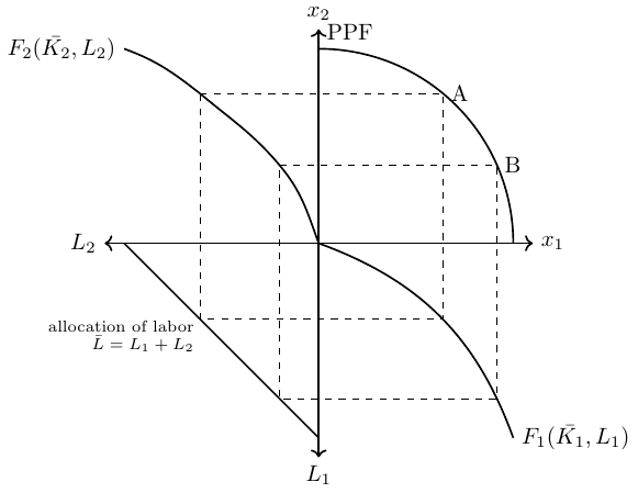
The two production functions, the fixed endowments and the distribution of labor determine the aggregate PPF. The PPF, which is the product of two production functions (\(F_1\) and \(F_2\)), is shown in Figure 35.2. The figure shows, for both production points A and B, how the mobile factor of production, labor, must be reallocated from sector 2 to sector 1 in order to produce more of good 1 in production point B. The second and fourth quadrants show the respective production functions of sectors 1 and 2.
35.3 Equillibrium in autarky:
- Depending on a country’s demand for good 1 and 2 a production point on the PPF is chosen at which it must hold that the slope of the PPF curve and the price relation (that is, relation of marginal product of labor in sector 1 and sector 2) must be equal: \[\begin{align*} \frac{p_1}{p_2}=\frac{\frac{\partial F_2}{\partial L_2}}{\frac{\partial F_1}{\partial L_1}} \end{align*}\]
- What can we say about the rents of the production factors?
- From the assumption of perfect competition it follows that firms do not make a positive profit in equilibrium, \(\pi\overset{!}{=}0\). Thus, the equilibrium wage for sectors \(g \in \{1, 2\}\) are given by the profit maximizing of firms \[\begin{align*} \pi_g&=p_g\cdot F_g(\bar{K_g},L_g)-w_gL_g-r_gK_g\\ \frac{\partial \pi_g}{\partial L_g}&= p_g\cdot \frac{\partial F_g}{\partial L_g}-w_g\overset{!}{=}0 \qquad \Leftrightarrow w_g=p_g\frac{\partial F_g}{\partial L_g} \end{align*}\]
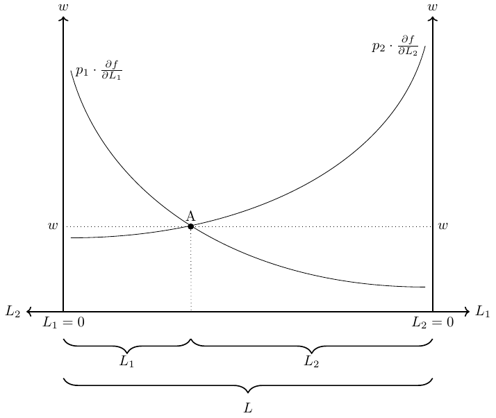
- We know that labor can move freely between sectors and an equilibrium exists when there are no incentives to move any further. That is the case when wages in both sectors are equal, \(w_1=w_2\). Thus, we can express wages in terms of purchasing power in units of good 1 as follows: \[\begin{align*} w_1&=p_1\frac{\partial F_1}{\partial L_1}\qquad \text{ and } \qquad w_2=p_2\frac{\partial F_2}{\partial L_2}\\ \Rightarrow w&=p_1\frac{\partial F_1}{\partial L_1}=p_2\frac{\partial F_2}{\partial L_2}\\ \Leftrightarrow \frac{w}{p_1}&=\frac{\partial F_1}{\partial L_1}\\ \Leftrightarrow \frac{w}{p_2}&=\frac{\partial F_2}{\partial L_2} \end{align*}\]
- Figure 35.3 presents the equilibrium wage and the optimal allocation of labor into sector 1 and 2.
35.4 Equilibrium under free trade:
Assume the price of good 1 and good 2 increase due to a trade opening in the same proportion. What happens with the real wage and the real incomes of capital-1 and capital-2 owners? The answer is: no real changes occur.
- The wage rate, \(w\), rises in the same proportion as the prices, so the real wages are unaffected. In Figure 35.3 this can be shown by shifting both curves upward.
- The real incomes of capital owners also remain the same because there will be no reallocation of labor across sectors.
Now, assume only the price of good 1 rises for 10% while \(p_2\) remains fixed, \(\frac{p'_1}{p_2}>\frac{p_1}{p_2}\). What happens with the real wage and the real incomes of capital-1 and capital-2 owners? The answer is: some win, some lose, and some maybe win.
Wages:
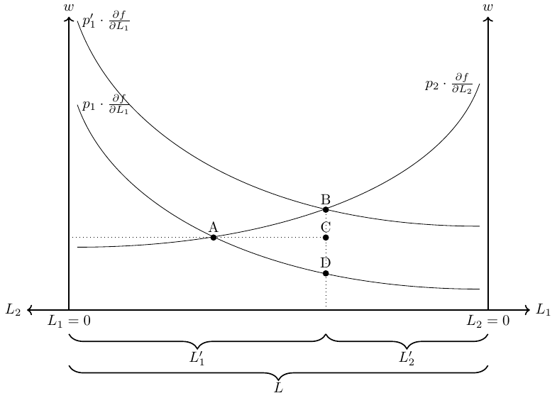
- \(p_1\frac{\partial F_1}{\partial L_1}\) rises and hence labor reallocates from sector 2 to sector 1 (\(L_1\uparrow\) and \(L_2\downarrow\)). This is shown in Figure 35.4.
- This reallocation of labor has some implications for the real wages measured in purchasing power of good 1 and 2, respectively:
- The price of good 1 has increased by 10%, the wage has however increased by less than 10% (compare the length of BC and BD in the figure), whereas the price for food stays constant.
- Thus, the purchasing power in buying good 2 increased, whereas the purchasing power in buying good 1 decreased. Hence, workers gain when buying good 2 but lose when buying good 1
- Overall, the welfare effect from real wages is unclear and depends on preferences.
Owner of capital-1:
- Owners of capital-1 receive a 10% higher price on their products but have to pay a less than 10% higher wage.
- Overall, capital-1 owners gain from free trade because they can employ more workers (at a higher price) now.
Owner of capital-2:
- Owner of capital-2 receive the same price on their products but have to pay a higher wage.
- Overall, capital-2 owners lose from free trade because they can employ less workers at a higher price now.
You can think of capital specific to the production of manufacturing goods (good 1) and land specific to the production of food sector goods (good 2)↩︎