33 Comparative advantage
Source: National Portrait Gallery
David Ricardo (1772-1823), one of the most influential economists of his time, had a simple idea that had a major impact on how we think about trade. In Ricardo (1817), he argued that bilateral trade can be a positive-sum game for both countries, even if one country is less productive in all sectors, if each country specializes in what it can produce relatively best.
He introduced the theory of comparative advantage that is still an important corner stone of the modern theory of international trade1 The theory is also known as the Ricardian model. It refers to the ability of one party (an individual, a firm, or a country) to produce a particular good or service at a lower opportunity cost than another party. In other words, it is the ability to produce a product with the highest relative efficiency, given all other products that could be produced. In contrast, an absolute advantage is defined as the ability of one party to produce a particular good at a lower absolute cost than another party.

As shown in Figure 33.2, the concept of comparative advantage is quite simple. Two parties can increase their overall productivity by sharing the workload based on their respective comparative advantages. Once they have achieved this increase in productivity, they must agree on how to divide the resulting output. Of course, both parties must benefit compared to a scenario in which they work independently.
33.1 Defining absolute and comparative advantages
A subject (country, household, individual, company) has an absolute advantage in the production of a good relative to another subject if it can produce the good at lower total costs or with higher productivity. Thus, absolute advantage compares productivity across subjects but within an item.
A subject has a comparative advantage in the production of a good relative to another subject if it can produce that good at a lower opportunity cost relative to another subject.
Let me explain the idea of the concept of comparative advantage with some examples:
Old and young
Two women live alone on a deserted island. In order to survive, they have to do some basic activities like fetching water, fishing and cooking. The first woman is young, strong and educated. The second is older, less agile and rather uneducated. Thus, the first woman is faster, better and more productive in all productive activities. So she has an absolute advantage in all areas. The second woman, in turn, has an absolute disadvantage in all areas. In some activities, the difference between the two is large; in others, it is small. The law of comparative advantage states that it is not in the interest of either of them to work in isolation: They can both benefit from specialization and exchange. If the two women divide the work, the younger woman should specialize in tasks where she is most productive (for example, fishing), while the older woman should focus on tasks where her productivity is only slightly lower (for example, cooking). Such an arrangement will increase overall production and benefit both.
The lawyer’s typist
The famous economist and Nobel laureate Paul Samuelson (1915-2009) provided another example in his well-received textbook of economics, as follows: Suppose that in a given city the best lawyer also happens to be the best secretary. However, if the lawyer focuses on the task of being a lawyer, and instead of practicing both professions at the same time, hires a secretary, both the lawyer’s and the secretary’s performance would increase because it is more difficult to be a lawyer than a secretary.2
33.2 Autarky: An example of two different persons
Assume that A and B want to produce and consume \(y\) and \(x\) respectively. Because of the complementarity of the two goods, each must be consumed in combination with the other. The utility function of both persons is \(U_{\{A;B\}}=min(x,y)\). Both persons work for 4 time units, that is, their units of labor are \(L_A=L_B=4\). A needs 1 units of labor to produce one unit of good \(y\) and 2 units of labor to produce one unit of good \(x\). B needs \(\frac{4}{10}=0.4\) units of labor to produce one unit of good \(y\) or good \(x\). Thus, their labor input coefficients, which measure the units of labor required by a subject to produce one unit of good, are \(a^A_y=1, a^A_x=2, a^B_y=0.4, a^B_x=0.4\):
| input coefficient (\(a\)) | A | B |
|---|---|---|
| Good \(y\) | 1 | 0.4 |
| Good \(x\) | 2 | 0.4 |
Spending all her time in the production of \(y\), A can produce \(\frac{L_A}{a_y^A}=\frac{4}{1}=4\) units of \(y\) and B can produce \(\frac{L_B}{a_y^B}=\frac{4}{0.4}=10\) units of \(y\). Spending all her time in the production of \(y\), A can produce \(\frac{L_A}{a_x^A}=\frac{4}{2}=2\) units of \(x\)and B can produce \(\frac{L_B}{a_x^B}=\frac{4}{0.4}=10\) units of \(x\). Knowing this, we can easily draw the production possibility frontier curves (PPF) of person A and B as shown in Figure 33.3.
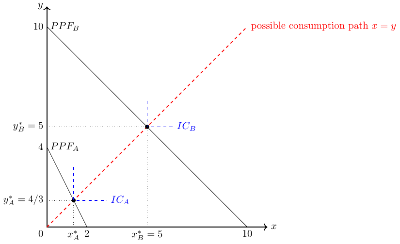
In autarky, both person maximize their utility: Individual A can consume \(\frac{4}{3}\) units of each good and individual B can consume \(5\) units of each good. The respective indifference curves are drawn in dashed blue lines in Figure 33.3.
33.2.1 Can person A and B improve their maximum consumption with cooperation?
Let us assume the two persons come together and try to understand how they can improve by jointly deciding which goods they should produce. If we assume that both persons redistribute their joint production so that both have an incentive to share and trade, we can concentrate on the total production output. Their joint PPF curve can then be drawn in two ways:
- Person A specializes in good \(x\), then the joint production possibilities are presented in Figure 33.4.
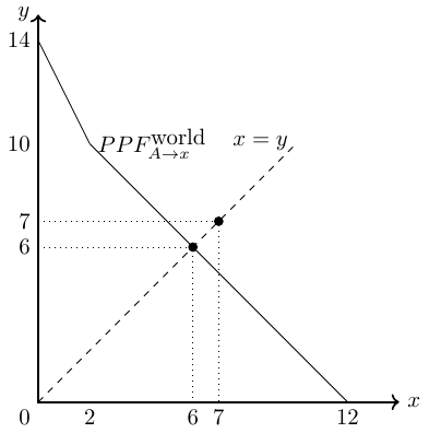
If A produces only good \(x\), as shown in Figure 33.4, we see that A and B can consume a total of 6 units of goods \(x\) and \(y\). This is less in total than in autarky, where A can consume \(\frac{4}{3}\) units of each good and person B can consume \(5\) units of each good, giving a combined consumption of \(\frac{19}{3}=6,\bar{6}\).
- Person A specializes in good \(y\), then the joint production possibilities are presented in Figure 33.5.
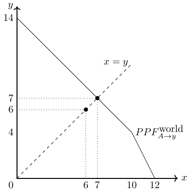
If A produces only good \(y\), as shown in Figure 33.5, we see that A and B can consume a total of 7 units of goods \(x\) and \(y\). Thus, both can be better off compared to autarky, since the total quantity distributed is larger. Thus, we have an Pareto improvement here because at least one person can be better off compared to autarky.
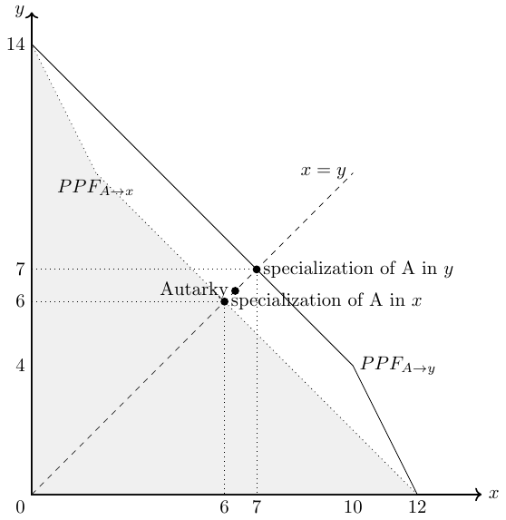
In Figure 33.6, the three possible consumption scenarios are marked with a dot and the PPFs of person A specializing in the production of good \(x\) (\(PPF_{A\rightarrow x}\)) or good \(y\) (\(PPF_{A\rightarrow y}\)) are also drawn. The scenario with person A specializing in the production of good \(y\) is the output maximizing solution.
33.2.2 Optimal production in cooperation
In order to produce the most bundles of both goods, the optimal cooperative production is
| production in cooperation | A | B |
|---|---|---|
| Good \(y\) | 4 | 3 |
| Good \(x\) | 0 | 7 |
33.2.3 Check for absolute advantage
Employing 10 units of labor B can produce more of both goods and hence has an absolute advantage in producing \(x\) and \(y\). Formally, we can proof this by comparing the input coefficients of both countries in each good:
| absolute advantage | A | B | ||
|---|---|---|---|---|
| Good \(y\) | \(a_y^A=1\) | > | \(0.4=a_y^B\) | \(\Rightarrow\) B has an absolute advantage in good \(y\) |
| Good \(x\) | \(a_x^A=2\) | > | \(0.4=a_x^B\) | \(\Rightarrow\) B has an absolute advantage in good \(x\) |
33.2.4 Check for comparative advantage
The slope of the PPFs represent the marginal rate of transformation, the terms of trade in autarky and the opportunity costs of a country. The opportunity costs are defined by how much of a good \(x\) (or \(y\)) a person (or country) has to give up to get one more of good \(y\) (or \(x\)). For example, A must give up \(\frac{a_x^A}{a_y^A}=\frac{1}{2}=0.5\) of good \(x\) to produce one more of good \(y\). Thus, A’s opportunity costs of producing one unit of \(y\) is the production foregone, that is, a half good \(x\). All opportunity costs of our example are:
| opportunity costs of producing … | A | B |
|---|---|---|
| …1 unit of good \(y\): | \(\frac{a_y^A}{a_x^A}=\frac{1}{2}=0.5\) (good x) | \(\frac{a_y^B}{a_x^B}=\frac{0.4}{0.4}=1\) (good x) |
| …1 unit of good \(x\): | \(\frac{a_x^A}{a_y^A}=\frac{2}{1}=2\) (good y) | \(\frac{a_x^B}{a_y^B}=\frac{0.4}{0.4}=1\) (good y) |
Person A has a comparative advantage in producing good \(y\) since A must give up less of good \(x\) to produce one unit more of good \(y\) than person B must. In turn, Person B has a comparative advantage in producing good \(x\) since B must give up less of good \(y\) to produce one unit more of good \(x\) than person B must give up of good \(y\) to produce one unit more of good \(x\). Thus, every person has a comparative advantage and if both would specialize in producing the good in which they have a comparative advantage and share their output they can improve their overall output as was shown in Figure 33.6.
An alternative and more direct way to see the comparative advantages of A and B, respectively, is by comparing the two input coefficients of A with the two input coefficients of B: \[\begin{align*} \frac{a^A_y}{a^A_x} &\lesseqqgtr \frac{a^B_y}{a^B_x} \quad \Rightarrow \quad \frac{1}{2} <\frac{0.4}{0.4}. \end{align*}\] Thus, A has a comparative advantage in \(y\) and B in \(x\).
33.2.5 Trade structure and consumption in cooperation
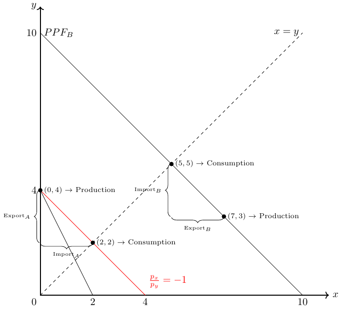
If A specializes in the production of \(y\), she must import some of good \(y\), otherwise she cannot consume a bundle of both goods as desired. In turn, B wants to import some of the good \(y\). B will not accept to consume less than 5 bundles of \(y\) and \(x\) as this was his autarky consumption. Thus, B wants a minimum of 2 units of good \(y\) from A. A will not accept to give more than \(4-\frac{4}{3}=2\frac{2}{3}\) items of good \(y\) away and he wants at least \(\frac{4}{3}\) items of good \(x\). Overall, we can define three trade scenarios:
- All gains from cooperation goes to A (see Figure 33.7 and Table 33.1);
- All gains from cooperation goes to B (see Table 33.2); or
- The gains from specialization and trade are shared by A and B with a trade structure between the two extreme scenarios.
| Consumption | A | B |
|---|---|---|
| Good \(y\) | 2 | 5 |
| Good \(x\) | 2 | 5 |
| Trade | A | B |
|---|---|---|
| Good \(y\) | -2 | 2 |
| Good \(x\) | 2 | -2 |
| Consumption | A | B |
|---|---|---|
| Good \(y\) | \(\frac{4}{3}\) | \(5\frac{2}{3}\) |
| Good \(x\) | \(\frac{4}{3}\) | \(5\frac{2}{3}\) |
| Trade | A | B |
|---|---|---|
| Good \(y\) | \(-\frac{2}{3}\) | \(\frac{2}{3}\) |
| Good \(x\) | \(\frac{4}{3}\) | \(-\frac{4}{3}\) |
Each of the three cases yield a Pareto-improvement, that is, none gets worst but at least one gets better by mutually decide on production and redistribute the joint output. In the real world, however, it is often difficult for countries to cooperate and decide mutually on production and consumption. In particular, it is practically difficult to enforce redistribution of the joint outcome so that everyone is better off. So let’s examine whether there is a mechanism that yields trade gains for both trading partners.
33.3 The Ricardian model
To understand the underlying logic of the argument, let us formalize and generalize the situation of two subjects and their choices for production and consumption.
In particular, the Ricardian Model build on the following assumptions:
- 2 subjects (A,B) can produce 2 goods (x,y) with
- technologies with constant returns to scale. Moreover,
- production limits are defined by \(y^i Q_y^i+ a_x^i Q_x^i=L^i\)$, where \(a^i_j\) denotes the unit of labor requirement for person \(i \in \{A,B\}\) in the production of good \(j\in \{x,y\}\) and \(Q^i_j\) denotes the quantity of good \(j\) produced by person \(i\), and \(Q^i_j\) the quantity of good \(j\) produced by person \(i\) and \(Q^i_j\) the quantity of good \(j\) produced by person \(i\). (Imagine they both work 4 hours).
- Let \(a^i_j\) denote the so-called labor input coefficients, that is, the units of labor required by a person \(i \in \{A,B\}\) to produce one unit of good \(j\in \{x,y\}\).
- Suppose further that person B requires fewer units of labor to produce both goods, that is, \(a^A_y>a^B_y\) and \(a^A_x>a^B_x\), and that
- a comparative advantage exists, that is, \(\frac{a^B_y}{a^B_x} \neq \frac{a^A_y}{a^A_x}\).
33.4 Distribution of welfare gains
The Ricardo theorem tells us nothing about the precise distribution of welfare gains. In this section, I will show that the distribution of welfare gains is the result of relative supply and demand in the world.
To illustrate this, consider Ricardo’s famous example4 of two countries (England and Portugal) that can produce cloth \(T\) and wine \(W\) with different input requirements, namely:
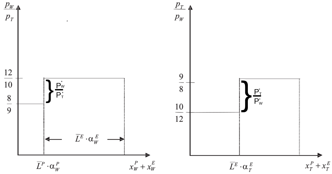
\[\begin{align*} \frac{p^P_W}{p^P_T}=\frac{a^P_W}{a^P_T}=\frac{8}{9}<\frac{12}{10}=\frac{a^E_W}{a^E_T}= \frac{p^E_W}{p^E_T} \end{align*}\] Thus, England has an absolute disadvantage in the production of both goods, but England has a comparative advantage in the production of cloth and Portugal has a comparative advantage in the production of wine. Let us further assume that both countries are similarly endowed with labor, \(\bar{L}\). Then we can calculate the world supply of cloth and wine given relative world prices, \(\frac{p_T}{p_W}\). Since we know that Portugal will only produce wine if the price of wine relative to cloth is above \(\frac{p_W}{p_T}=\frac{8}{9}\) and England will only produce wine if the price of wine relative to cloth is above \(\frac{p_W}{p_T}=\frac{12}{10}\), we can draw the relative world supply of goods as shown in the left panel of Figure 33.8. Note that \(\alpha\) in the figure means \(\frac{1}{a}\). Similarly, we can draw in the world supply of clothes, shown in the left panel of Figure 33.8.
Whether both countries specialize totally in the production of one good, or only one country does so depends on world demand for both goods at relative prices. Since we know from the Ricardo Theorem that the world market price relation, \(\frac{p^{*}_T}{p^{*}_W}\), must be between the two autarky price relations: \[\begin{align}
\frac{p^P_T}{p^P_W}>\frac{p^{*}_T}{p^{*}_W}> \frac{p^E_T}{p^E_W}.
\end{align}\] If world demand for cloth would be sufficiently high to have a world price of \[\frac{p^P_T}{p^P_W}=\frac{9}{8}\] Portugal would not gain from trade. On the contrary, if world demand for wine would be sufficiently high to have a world price of \[\frac{p^P_T}{p^P_W}=\frac{10}{12}\] England would not gain from trade. Thus, the price span between \(\frac{10}{12}\) and \(\frac{9}{8}\) says us which country gains from trade. For example, at a world price of \[\frac{p^{*}_T}{p^{*}_W}=1\] about 57%
\[\begin{align}
\left[\frac{\left(1-\frac{10}{12}\right)}{\left(\frac{9}{8}-\frac{10}{12}\right)}\approx 0.57 \right]
\end{align}\] of the gains through trade will be distributed to Portugal and about 43% will be distributed to England.
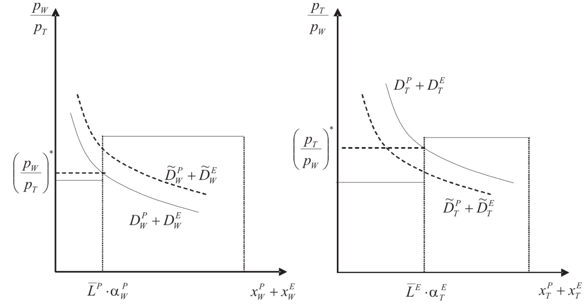
In Figure 33.9, I show two demand curves of the World. The dashed demand curve represents a world with a relative strong preference on wine and the other demand curve represents a relative strong demand for cloth. Since Portugal has a comparative advantage in producing wine, they would happy to live in a world where demand for wine is relatively high, whereas the opposite holds true for England.
Exercise 33.9 Bike and tires
Consider two countries, \(A\) and \(B\). Both have a labor endowment of 24, \(L^A=L^B=24\). In both countries two goods can be produced: bikes, which are denoted by \(y\), and bike tires, which are denoted by \(x\). Assume that the two goods can only be consumed in bundles of one bike and two bike tires. The following graph illustrates the production possibility (PPF) curve of both countries in autarky, i.e, country A and B do not trade with each other.
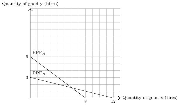
- How many complete bikes, that is, one bike with two tires, can be consumed in autarky in country A and B, respectively. Draw the production points for country A and B into the figure. (A calculation is not necessary.)
- Calculate —for both countries—the input coefficients, \(a\), that is, the units of labor needed to produce one unit of good \(y\) and good \(x\), respectively. Fill in the four input coefficients in the following table:
| Country A | Country B | |
|---|---|---|
| Good y (bikes) | (\(~~~~~~~\)) | (\(~~~~~~~\)) |
| Good x (bike tires) | (\(~~~~~~~\)) | (\(~~~~~~~\)) |
- Fill in the ten gaps (\(~~~~~~~\)) in the following text:
If we assume that both countries specialize completely in the production of the good at which they have a comparative advantage and trade is allowed and free of costs, then
country A produces (\(~~~~~~~\)) units of bikes and (\(~~~~~~~\)) units of tires and
country B produces (\(~~~~~~~\)) units of bikes and (\(~~~~~~~\)) units of tires.
Moreover, since both countries aim to consume complete bikes, that is, one bike with two tires,
country A exports (\(~~~~~~~\)) units of (\(~~~~~~~\)) and imports (\(~~~~~~~\)) units of (\(~~~~~~~\)) and
country B exports (\(~~~~~~~\)) units of (\(~~~~~~~\)) and imports (\(~~~~~~~\)) units of (\(~~~~~~~\)).
Under free trade - country A can consume (\(~~~~~~~\)) complete bikes and - country B can consume (\(~~~~~~~\)) complete bikes.
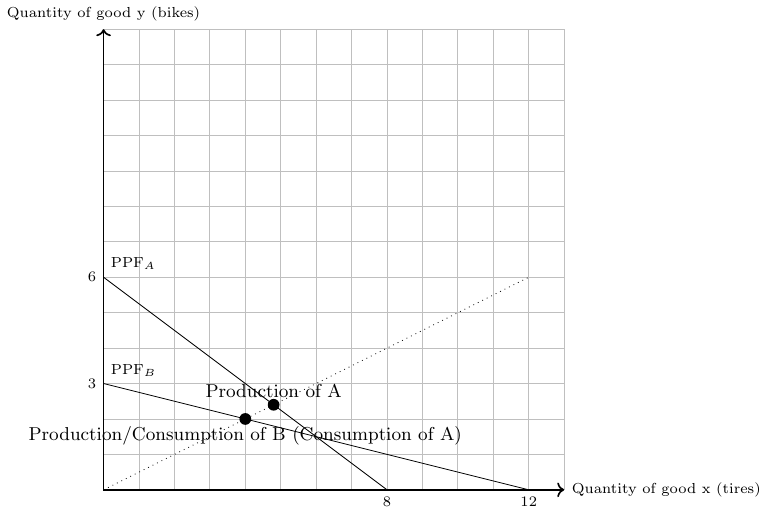
- Both countries can consume 2 complete bikes, see Figure 33.11.
| Country A | Country B | |
|---|---|---|
| Good \(y\) (bikes) | 24:6=4 | 24:3=8 |
| Good \(x\) (bike tires) | 24:8=3 | 24:12=2 |
- If we assume that both countries specialize completely in the production of the good at which they have a comparative advantage and trade is allowed and free of costs, then
- country A produces 6 units of bikes and 0 units of tires and
- country B produces 0 units of bikes and 12 units of tires.
Moreover, since both countries aim to consume complete bikes, i.e., one bike with two tires,
- country A exports 3 units of bikes and imports 6 units of tires and
- country B exports 6 units of tires and imports 3 units of bikes.
Under free trade
- country A can consume 3 complete bikes and
- country B can consume 3 complete bikes.
Actually, strictly speaking, this is not correct, since the original description of the idea can already be found in Torrens (1815). However, David Ricardo formalized the idea in his 1817 book using a convincing and simple numerical example. For more information on this, as well as a great introduction to the Ricardian model and more, I recommend Suranovic (2012).↩︎
In the first eight editions the example comprised a male lawyer who was better at typing than his female secretary, but who had a comparative advantage in practising law. In the ninth edition published 1973, both lawyer and secretary were assumed to be female (see Backhouse & Cherrier, 2019). Unfortunately, women are still discriminated against in introductory economics textbooks (see Stevenson & Zlotnik, 2018).↩︎
In order to see that the relative prices within a country equals the relative productivity parameters, consider that nominal income of labor in producing good \(j\in \{x,y\}\), \(w_jL^i_j\), must equal the production value, that is, \(p_j^ix_j^i\): \[ w_jL^i_j=p_j^ix_j^i. \] Setting \(w_j=1\) as the numeraire and re-arranging the equation, we get \[ p_j^i=\frac{L_j^i}{x_j^i}=a_j^i. \] ↩︎
The example is explained by Suranovic (2012) in greater detail.↩︎