30 International investments
Investing, whether through holding a currency or storing purchasing power, is inherently speculative, regardless of whether the investment is domestic or international. When you hold a foreign currency, it’s crucial to acknowledge that its value can both appreciate and depreciate. Currency values can fluctuate significantly over time due to factors such as economic policy, market sentiment, and global events. In the following sections, I will present a framework to help understand the key determinants of the rate of return on your investment. As illustrated in Figure 30.1, we will explore how a country’s interest rates, trade balances, price levels, and exchange rates are interconnected and must be analyzed together, rather than in isolation.
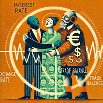
Source: Generated using OpenAI (2025).
30.1 Foreign exchange reserves
Currencies serve as a store of value, an important function in the financial world. Foreign exchange reserves are assets held on reserve by a central bank in foreign currencies, which can include bonds, treasury bills, and other government securities. The primary purpose of holding foreign exchange reserves is to manage the exchange rate of the national currency and ensure the stability of the country’s financial system.
Accordingly to the Currency Composition of Official Foreign Exchange Reserves (COVER) database of the International Moentary Fund (IMF), the total foreign exchange reserves in Q3 2023 had been 11,901,53 billion U.S. Dollar. That is, $ 11,901,530,000,000!
The size of a country’s foreign exchange reserves can be influenced by various factors, including its balance of trade, exchange rate policies, capital flows, and the overall health of its economy. While having substantial reserves is generally seen as a sign of economic strength and stability, excessively accumulating reserves can also indicate underlying economic imbalances or protectionist policies.
30.2 Three components of the rate of return
An investment usually has different characteristics such as the default risk, opportunities, and liquidity. These characteristics and individual preferences are important to decide which investment is superior. In this course, however, we mostly refrain from discussing sophisticated features of investments here. We focus on the most important feature of an investment, that is, the rate of return. In particular, three components are important to calculate the rate of return:
30.2.1 Interest rate
The interest rate of an investment is a crucial factor that determines the return earned on invested capital over a specific period. It represents the percentage of the initial investment that is paid back to the investor as interest or profit. Formally, we can write: \[ \underbrace{I_{t-1}}_{\text{investment in {t-1}}} \cdot\quad \underbrace{(1+i)}_{1+\text{interest rate}} = \underbrace{I_{t}}_{\text{payout amount in t}} \tag{30.1}\] where \(I\) denotes the value of an asset measured in € in the respective time period \(t\).
30.2.2 Exchange rate
When investing in assets denominated in foreign currencies, investors need to convert their domestic currency into the foreign currency at the prevailing exchange rate. After the investment has been paid out in the foreign country, the investor must convert the foreign currency back to his home currency. Thus, the initial cost of the investment and the subsequent returns are influenced by the exchange rate at the beginning and the end of the investment.
Formally, we can write if the an investment takes in foreign country, that is, Turkey between \(t-1\) and \(t\): \[ I^{\text{€}}_{t-1}\cdot E_{t-1}^{\frac{\text{₺}}{\text{€}}} \cdot E_{t}^{\frac{\text{€}}{\text{₺}}}= I_{t}^{\text{€}} \tag{30.2}\]
30.2.3 Inflation
Inflation refers to the quantitative measure of the rate at which prices, represented by a basket of goods and services, increase within an economy over a specific period. Conversely, negative inflation is termed deflation. Mathematically, inflation can be defined as follows:
\[ \pi = \frac{P_t - P_{t-1}}{P_{t-1}} = \frac{P_t}{P_{t-1}} - 1 \]
Where \(\pi\) represents the inflation rate and \(P_t\) denotes the price at time \(t\). When inflation affects all prices, it also impacts the value of assets in which investors are invested. This relationship can be expressed as:
\[ I_t = I_{t-1} \cdot (1+\pi) \tag{30.3}\]
30.3 Rate of return of an investment abroad
The rate of return, \(r\), is the growth rate of an investment over time and can be described as follows: \[\begin{align*} r=& \frac{I^{\text{€}}_t-I_{t-1}^{\text{€}}}{I_{t-1}^{\text{€}}}=\frac{I^{\text{€}}_t}{I^{\text{€}}_{t-1}}-1, \end{align*}\]
Combining Equation 30.1, Equation 30.2, and Equation 30.3, we can describe the value of our investment in period \(t\) as follows: \[ I_{t}^{\text{€}}= I_{t-1}^{\text{€}} \cdot (1+i^{*}) \cdot E_{t-1}^{\frac{\text{₺}}{\text{€}}} \cdot E_{t}^{\frac{\text{€}}{\text{₺}}} \cdot (1+\pi^{*}), \tag{30.4}\] where \(I_{t-1}^{\text{€}}\) denotes the initial investment, \(i^{*}\) denotes the interest rate abroad and \(\pi^{*}\) the inflation abroad. Dividing by \(I_{t-1}^{\text{€}}\) and subtracting \(1\) from both sides of Equation 30.4, we see that the rate of return for an investment abroad, \(r^{*}\), has three determining factors, that are: interest rate \((1+i^*)\), inflation \((1+\pi)\), and the change of exchange rates over time \((E_{t-1}^{\frac{\text{₺}}{\text{€}}} \cdot E_{t}^{\frac{\text{€}}{\text{₺}}})\): \[\begin{align*} \underbrace{\frac{I_{t}^{\text{€}}}{I_{t-1}^{\text{€}}}-1}_r^*&= (1+i^{*})\cdot (1+\pi^{*}) \cdot \underbrace{E_{t-1}^{\frac{\text{₺}}{\text{€}}} \cdot E_{t}^{\frac{\text{€}}{\text{₺}}}}_\alpha -1 \end{align*}\] \[ r^*= (1+i^{*})\cdot (1+\pi^{*}) \cdot \alpha -1 \tag{30.5}\] with
- \(\alpha=1\) if the exchange rate does not change over time and
- \(\alpha>1\) if the home currency € depreciates or
- \(\alpha<1\) if the home currency € appreciates.
So the exchange rate changes over time work as a third factor of your rate of return.
By assuming no inflation (\(\pi^{*}=0\)), we can write
\[
\begin{aligned}
r^*&=(1+i^{*}) \cdot \alpha -1\\
\Leftrightarrow r^*&=\alpha +\alpha i^{*} -1.
\end{aligned}
\tag{30.6}\] Reorganizing Equation 30.6 helps to interpret it. Firstly, let us expand the right hand side of this equation adding and subtracting \(i^*\) which obviously does not change the sum of the right hand side of the equation. Secondly, re-write the equation and thirdly, set \((\alpha-1)=w\): \[
\begin{aligned}
\Leftrightarrow r^*&=\alpha +\alpha i^{*}-1+i^*-i^*\\
\Leftrightarrow r^*&=\alpha-1+i^* +\alpha i^{*}-i^*\\
\Leftrightarrow r^*&=\underbrace{(\alpha -1)}_w+i^* +i^{*}\underbrace{(\alpha -1)}_w\\
\Leftrightarrow r^*&=w+i^* +i^{*}w
\end{aligned}
\tag{30.7}\]
This equation outlines the rate of return on an investment in a foreign country, influenced by two primary factors: \(i^*\) and \(w\).
Assuming that the product \(iw\) is very small, we can say that the rate of return equals approximately the interest rate plus the rate of depreciation: \[r^{*}=w+i^{*}.\] This approximation is often called the simple rule for \(r\).
30.4 The interest parity condition
Assume the rate of return is lower domestically than it is for investments abroad. Representing the foreign country with an asterisk \((*)\), this situation, where investing money abroad is more profitable, can be expressed as:
\[\begin{align*} r&<r^{*}. \end{align*}\] Given that domestically the rate of return, \(r\), equals the interest rate, \(i\), assuming zero inflation, and that the simple rule for an investment abroad is described by \(r^{*} = w + i^{*}\), we can rewrite the equation as: \[ i< w+i^{*}. \] What would happen if financial market actors became aware of this?
Market participants would likely convert their domestic currency into the foreign currency to invest abroad, increasing demand for the foreign currency. Consequently, the foreign currency would appreciate, becoming relatively more expensive. This implies that \(w\) is negative. This appreciation process halts when investing abroad no longer offers a higher return. If the attractiveness of investments is equalized, the FOREX is in equilibrium. The deposits of all currencies offer the same expected rate of return. In other words, in equilibrium the exchange rate, \(w\), assures that the rate of return from the home country, \(r\), is equal to the rate of return in any foreign country, denoted with an asterisk (\(*\)):
\[\begin{align} r&=r^{*}\\ i&= w + i^{*}\\ \end{align}\] \[ \Leftrightarrow w= i-i^{*} \tag{30.8}\]
The interest parity condition (Equation 30.8) enables us to analyze how variations in interest rates and expected exchange rates affect current exchange rates through comparative static analysis of the equation: \[ \frac{\partial w}{\partial i} > 0; \quad \frac{\partial w}{\partial i^*} < 0. \] This means:
- An increase in the domestic interest rate results in a positive change in the depreciation rate, leading to the depreciation of the domestic currency.
- An increase in the foreign interest rate causes a negative change in the depreciation rate, resulting in the appreciation of the domestic currency.
30.5 The theory in real markets: Unpegging the Swiss Franc
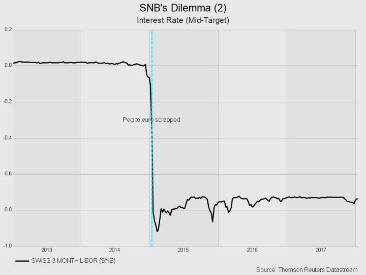
You might now question whether this theory of the interest parity condition truly holds in real-world markets. Analyzing international markets and the FOREX empirically is challenging due to the frequent occurrence of both large and small exogenous shocks on a global scale, each impacting market outcomes in various ways. Furthermore, market dynamics are often influenced by emotions and speculation rather than solely measurable facts. However, there are instances where the shocks are so significant that the fundamental forces driving the market become visible, even without a sophisticated empirical identification strategy that controls for confounding effects. The case study of the unexpected unpegging of the Swiss Franc serves as a poignant example. It vividly demonstrates that the principles underpinning the interest parity condition are not merely theoretical constructs but actively influence real market behaviors.
Until early 2015, the Swiss National Bank (SNB) had a policy goal to maintain the franc above the cap of 1.20 Francs per Euro, aiming to protect exporters and combat deflationary pressures. However, in a surprising move, the SNB unpegged the Franc in 2015. This decision was influenced by the appreciation pressure on the Franc, as many investors many investors wanted to store their assets in the Swiss Franc. Following the SNB’s announcement, the exchange rate plunged from 1.20 to 1.00 Franc per Euro \((E^{\frac{CHF}{\text{€}}})\), as illustrated in Figure 30.2 (a) Almost simultaneously, the interest rate experienced a decline, as depicted in Figure 30.2 (b). These developments align precisely with what the interest parity condition would predict, demonstrating its applicability in real-world financial market dynamics.
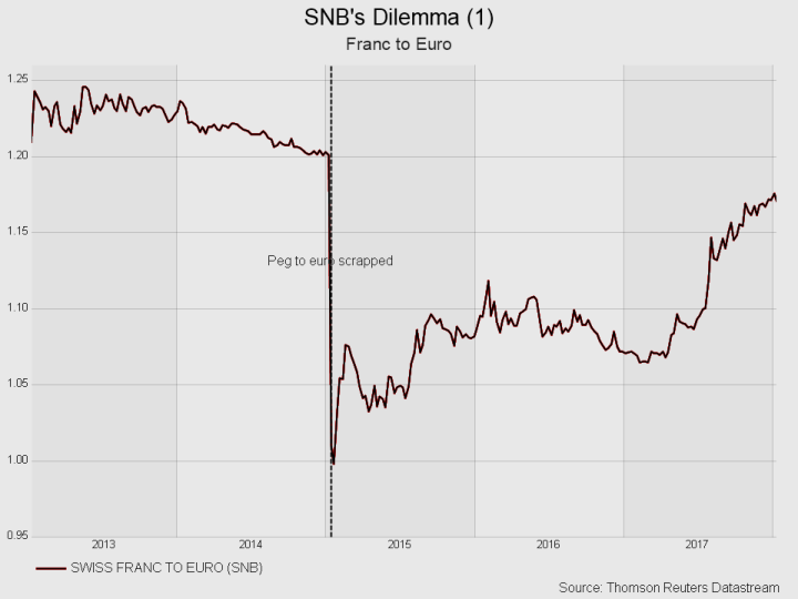
To analyze the relationship between changes in exchange rates and interest rates, we need to consider the interest parity assumption of Equation 30.8: \[ w= i-i^{*} \] where \[w=\frac{E_{t}^{\frac{\text{€}}{CHF}}}{E_{t-1}^{\frac{\text{€}}{CHF}}}-1.\] In January 2015, the exchange rate \(E^{\frac{CHF}{\text{€}}}\) decreased from 1.20 to 1.00. Alternatively, we can express this change in direct quotation, noting that the exchange rate \(E^{\frac{\text{€}}{CHF}}\) increased from \(E^{\frac{\text{€}}{CHF}}_{t-1}\approx \frac{1}{1.20}\approx 0.83\) to \(E^{\frac{\text{€}}{CHF}}_{t}\approx 1.00\), resulting in \[ w=\frac{E_{t}^{\frac{\text{€}}{CHF}}}{E_{t-1}^{\frac{\text{€}}{CHF}}}-1=\frac{1}{0.83}-1=0.20. \]
Since \(w > 0\), the fraction on the left-hand side of the interest rate parity equation must also be positive, as already mentioned. This implies that \[i - i^* > 0,\] which means that an interest rate spread must occur. This condition can occur if the foreign interest rate \(i^*\) decreases or the domestic interest rate \(i\) increases. In our observations, we can indeed see a pattern that is consistent with our theoretical expectations.
It is important to acknowledge that our theoretical framework simplifies the complex interplay of factors that influence both exchange rates and interest rates. Despite this simplification, the model highlights the key forces driving market dynamics. However, it is important to point out that the actual numbers may not perfectly match our theoretical predictions in quantitative terms, as shown in Figure Figure 30.3.
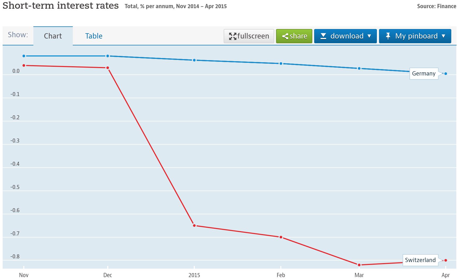
Source: Data are taken from the OECD and show the total, % per annum.
30.6 The Fisher Effect
The Fisher Effect is an economic theory proposed by economist Irving Fisher (1867-1947), which describes the relationship between (expected) inflation and both nominal and real interest rates.
According to the Fisher Effect, the nominal interest rate is equal to the sum of the real interest rate and the (expected) inflation rate. In formula terms, it is often expressed as: \[ r=i+\pi. \tag{30.9}\]
We can derive Equation 30.9 assuming that the exchange rate is stable over time \[ \left( E_{t-1}^{\frac{\text{€}}{\text{₺}}} =E_{t}^{\frac{\text{€}}{\text{₺}}} \Leftrightarrow \frac{E_{t-1}^{\frac{\text{€}}{\text{₺}}}}{E_{t}^{\frac{\text{€}}{\text{₺}}}}=1 \Leftrightarrow \alpha=1 \right) \] and using this in Equation 30.5, we get: \[\begin{align} r^*&= (1+i^{*})\cdot (1+\pi^{*}) \cdot \underbrace{\alpha}_{=1} -1 \\ \Leftrightarrow r=& i+ \pi+ \pi i \end{align}\] Assuming that the product \(\pi i\) is very small, we can say that the rate of return equals approximately the interest rate plus the inflation rate. This approximation shown in Equation 30.9 is often called the Fisher Effect.
Considering now cross-country differences in their rate of return, we can explain the rate of return spread by the inflation rate and the nominal interest rate spread as follows: \[r_{GER}-r_{TUR}= \pi_{GER}-\pi_{TUR} + i_{GER}-i_{TUR}. \tag{30.10}\]
We have learned in Section 30.4 (the interest parity condition) that the rate of return can differ only in the short run and will be equal across countries in the long run (\(r_{GER} - r_{TUR} = 0\)). Utilizing this concept in Equation 30.9, we can demonstrate that the nominal interest rates of countries will adjust to accommodate any changes in (expected) inflation, and vice versa:
\[i_{GER} - i_{TUR} = \pi_{GER} - \pi_{TUR}.\]
More information on the Fisher effect can be found here: Wikipedia (2025): Wikipedia entry to the Fisher Effect.