9 Supply and demand
Recommended readings:
Shapiro et al. (2022, ch. 3), Emerson (2019, ch. 11)
Shapiro, D., MacDonald, D., & Greenlaw, S. A. (2022). Principles of economics (3rd ed.). OpenStax. https://openstax.org/details/books/principles-economics-3e
Emerson, P. M. (2019). Intermediate microeconomics (O. S. University, Ed.; Versions 1st edition). Open Educational Resources. https://open.oregonstate.education/intermediatemicroeconomics
Learning objectives:
Students will be able to:
- Distinguish between quantity demanded and demand, and explain what determines demand.
- Distinguish between quantity supplied and supply, and explain what determines supply.
- Explain how demand and supply determine price and quantity in a market, and discuss the effects of changes in demand and supply.
9.1 What is a market?
A market is any arrangement that brings buyers and sellers together. A market might be a physical place or a group of buyers and sellers spread around the world who never meet. In this chapter, we study a competitive market that has so many buyers and sellers that no individual buyer or seller can influence the price. Quantity demanded is the amount of a good, service, or resource that people are willing and able to buy during a specified period at a specified price. The quantity demanded is expressed as an amount per unit of time, for example, the amount per day or per month. Supply and demand are the forces that make market economies work because they determine prices in a market economy. Prices, in turn, allocate the economy’s scarce resources. The model of the market based on supply and demand, like any other model, is based on a series of assumptions.
Klamer, A., McCloskey, D., & Ziliak, S. (2015). The economic conversation. https://www.theeconomicconversation.com
9.2 Demand
9.2.1 The law of demand
Other things remaining the same, if the price of the good rises, the quantity demanded of that good decreases. Conversely, if the price of the good falls, the quantity demanded of that good increases.
9.2.2 Demand schedule and demand curve
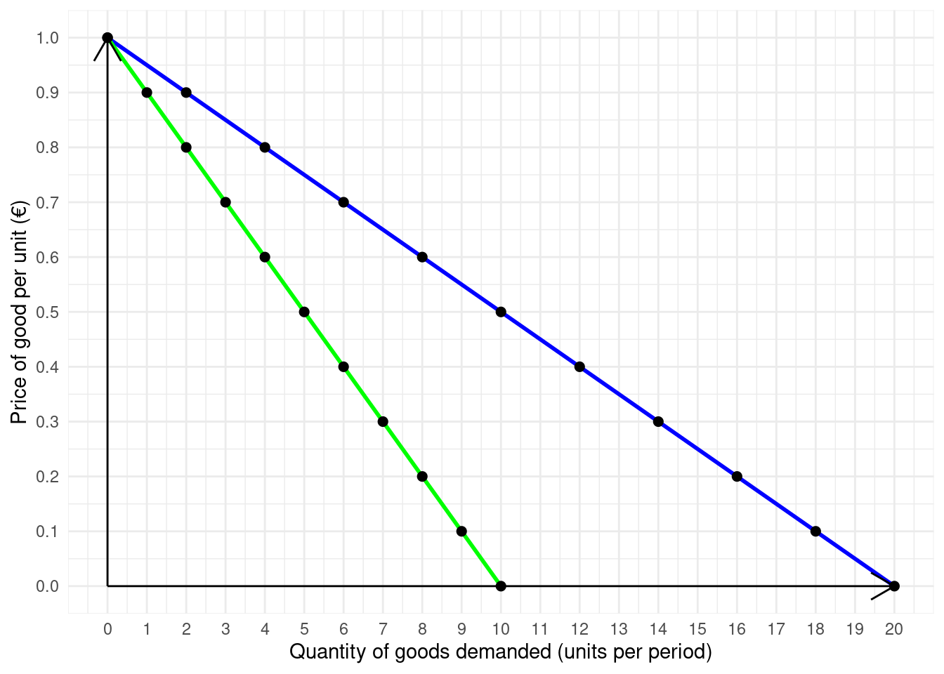
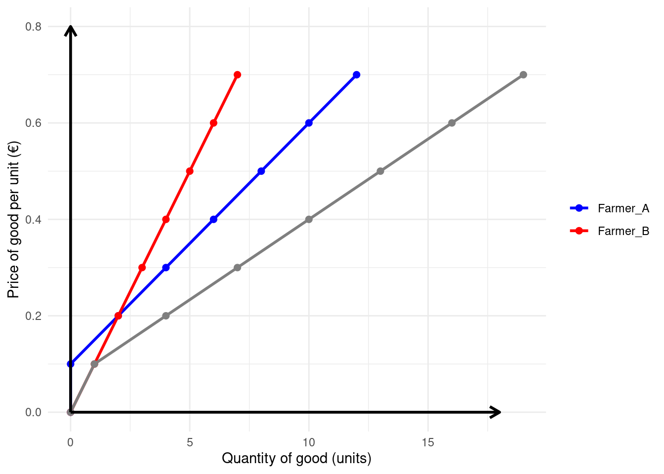
Demand is the relationship between the quantity demanded and the price of a good when all other influences on buying plans remain the same. Demand is illustrated by a demand schedule and a demand curve. The demand curve shows the relationship between price and quantity demanded. In Table 9.1 you see an example of a demand schedule for two individuals, A and B. This schedule is visualized in Figure 9.1.
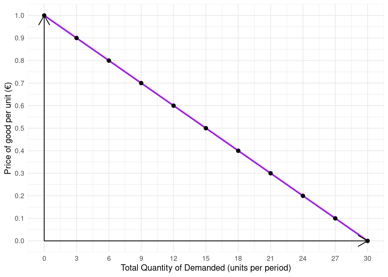
Market demand refers to the sum of all individual demands for a particular good or service. Graphically, individual demand curves are summed horizontally to obtain the market demand curve. The aggregated demand is visualized in Figure 9.2.
| Price of a per Unit (Euro) | Quantity Demanded by Person 1 (litres per month) | Quantity Demanded by Person 2 (units per period) | Total Quantity Demanded (units per period) |
|---|---|---|---|
| 0.00 | 20 | 10 | 30 |
| 0.10 | 18 | 9 | 27 |
| 0.20 | 16 | 8 | 24 |
| 0.30 | 14 | 7 | 21 |
| 0.40 | 12 | 6 | 18 |
| 0.50 | 10 | 5 | 15 |
| 0.60 | 8 | 4 | 12 |
| 0.70 | 6 | 3 | 9 |
| 0.80 | 4 | 2 | 6 |
| 0.90 | 2 | 1 | 3 |
| 1.00 | 0 | 0 | 0 |
9.2.3 Changes and shifts of demand
Movements along the demand curve are caused by a change in the price of the product. For example, if the price of a specific good changes, the quantity demanded will typically be altered by two effects: the income effect and the substitution effect:
- The income effect: Assuming that consumers’ incomes remain constant, a decrease in the price of a good allows them to purchase more of it with their available income.
- The substitution effect: If the price of one good is lower compared to other similar products, some consumers will choose to substitute the more expensive options with the now cheaper alternative, such as milk.
In section Section 11.2.5, I will discuss both the income and substitution effects in greater detail.
In contrast, changes in other factors that influence demand can result in a shift of the demand curve in a price-quantity diagram. A shift in the demand curve—either to the left or right—occurs when there is a change that affects the quantity demanded at every price level. Below is an incomplete list of factors that can cause demand curves to shift:
Income: The overall income of consumers greatly impacts their purchasing power. For normal goods, as income rises, the demand increases. Conversely, for inferior goods, demand decreases as income increases. For example, when consumers have higher incomes, they are less likely to purchase instant noodles (an inferior good) and may instead buy higher-quality meals.
Tastes and preferences: Changes in consumer preferences can shift demand. If health trends favor plant-based foods, demand for these products may rise, while demand for red meat may decline.
Consumer expectations: Expectations about future prices can influence current demand. If consumers expect that prices will rise in the future, they are more likely to purchase now, increasing current demand. Conversely, if they expect prices to drop, they may delay purchases, decreasing current demand.
Population and demographics: Changes in the number of consumers or their demographics can impact demand. For example, an aging population might increase the demand for healthcare products and services, while a growing youth demographic might boost demand for technology and entertainment products.
Price of related goods: When the price of a good rises, consumers may switch to other goods that offer similar benefits, known as substitutes. A substitute is a product that can be consumed in place of another. For example, apples and oranges are substitutes. If the price of butter increases, consumers may opt for margarine instead. In this scenario, the demand for margarine increases, while the demand for butter decreases. Conversely, demand can also be affected by changes in the prices of complementary goods—products that are often consumed together. A complement is a good that pairs well with another. For instance, sausages and mustard, or fish and chips are common complements. If the price of printers drops, the demand for ink cartridges might increase as more people purchase printers. Or, if the price of hot dogs rises, the demand for hot dog buns may decrease.
9.3 Types of goods
Goods can be classified based on how their demand reacts to changes in prices and consumer income. Here are some relevant types of goods:
9.3.1 Normal goods
A normal good is a good for which the demand increases as income increases or the price decreases.
9.3.2 Inferior goods
An inferior good is one for which the demand decreases as incomes increases.
Examples of inferior goods include budget brands, instant noodles, and second-hand clothing. When consumers have lower incomes, they may opt for these less expensive options, but as their income increases, they tend to switch to more expensive alternatives.
9.3.3 Giffen goods (Veblen goods):
A giffen good is a special type of good that increase in demand when its price rises, violating the basic law of demand. This phenomenon typically occurs for goods that are so essential that the consumer constitutes a significant portion of its budget and they buy even more it when the price increases as their inability to afford more expensive alternatives.
A Veblen good is a type of luxury good for which demand increases as the price increases, contrary to the law of demand. These goods serve as a status symbol. The higher price makes them more desirable to certain consumers who view these goods as markers of wealth or prestige. Examples include designer handbags and high-end cars.
Tip
Wikipedia. (2025b). Veblen good. https://en.wikipedia.org/wiki/Veblen_good
Wikipedia. (2025a). Giffen good. https://en.wikipedia.org/wiki/Giffen_good
Understanding these classifications is important in microeconomics as they help economists analyze consumer behavior, market trends, and the overall economy’s response to changes in income levels.
Exercise 9.3 Three demand curves
Use Figure 9.3 to draw a plot with three demand curves. Explain everything you show. One curve should represent an economy in an economic boom, one in an economic downturn, and one in between.
9.4 Supply
The law of supply states that, all else being equal: When the price of a good rises, the quantity supplied of that good increases and vice versa.
The quantity supplied is the amount of a good that sellers are willing and able to sell at a given price. In Table 9.2 an example of a supply schedule is shown that illustrates the relationship between the price of a good and the corresponding quantity supplied. The graphical representation of the relationship between the price of a good and the quantity supplied is visualized in Figure 9.4.
| Price of good per unit (Euro) | producer A | + | producer B | = | Market |
|---|---|---|---|---|---|
| 0.00 | 0 | + | 0 | = | 0 |
| 0.10 | 0 | + | 1 | = | 1 |
| 0.20 | 2 | + | 2 | = | 4 |
| 0.30 | 4 | + | 3 | = | 7 |
| 0.40 | 6 | + | 4 | = | 10 |
| 0.50 | 8 | + | 5 | = | 13 |
| 0.60 | 10 | + | 6 | = | 16 |
| 0.70 | 12 | + | 7 | = | 19 |
9.4.1 Changes and shifts of supply
The supply curve illustrates the quantities that producers are willing to offer for sale at various prices, while assuming that all other factors affecting their selling decisions remain constant. Any alteration in these additional factors—excluding price changes—results in a shift of the supply curve either to the left or the right.
Several key factors can cause shifts in the supply curve. These include the profitability of alternative goods in production and the prices of goods produced jointly. Advancements in technology can also influence supply, as can changes in the number of sellers in the market. Natural and social factors, such as weather conditions and evolving public attitudes, play a significant role as well. Furthermore, input prices—the costs associated with the factors of production—affect the supply. As production costs rise, the quantity supplied typically decreases. Expectations regarding future market conditions can also impact supply decisions, as can changes in resource prices. Higher resource and input prices generally elevate production costs, resulting in a reduced quantity supplied. Additionally, improvements in productivity—defined as output per unit of input—can lower costs and lead to an increase in supply.
A change in the price of one good can impact the supply of another good. This relationship occurs particularly in the context of goods that can be produced in place of one another, known as substitutes in production. These are goods that can be manufactured using similar resources, allowing producers to switch between them based on price fluctuations and market demands.
Overall, these dynamics illustrate the complex interplay of various factors that can influence how supply responds to changes in the market environment.
9.4.2 Market equilibrium
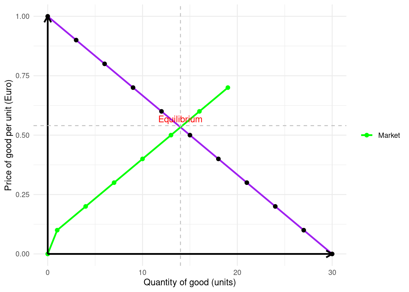
In economics, equilibrium refers to a situation where economic forces such as supply and demand are balanced. In the absence of external influences, the equilibrium values of economic variables remain unchanged.
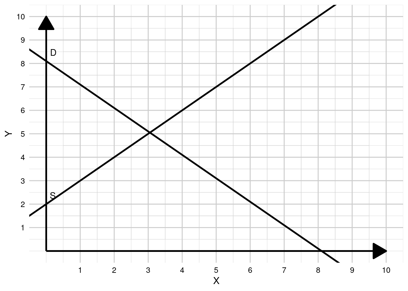
The price that balances quantity supplied and quantity demanded is called the equilibrium price. Graphically, this is the price at which the supply and demand curves intersect. The quantity that comes along the equilibrium price is called the equilibrium quantity. That is visualized in Figure 9.5.
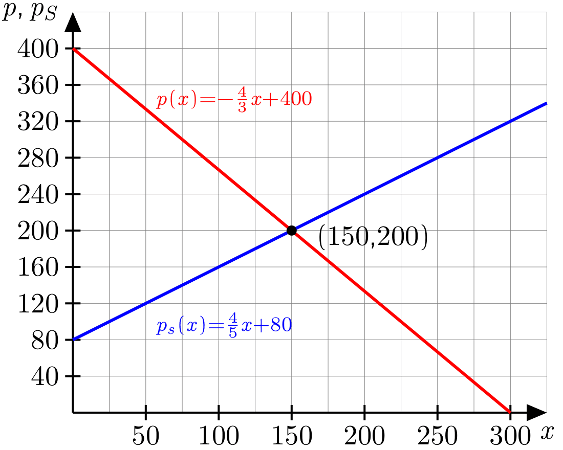
Exercise 9.5 After the visual determination of the equilibrium market price and quantity, calculate the equilibrium market price and quantity assuming the demand function:
\[x(p) = -\frac{3}{4}p + 300\]
and the supply function
\[x_S(p) = \frac{5}{4}p - 100.\]
Addtionally, draw the two functions and mark the equilibrium.
TipSolution
To formally calculate the equilibrium market price and quantity using the given demand and supply functions, you can set the two equations equal to each other and solve for the price (p). Here’s how it can be represented mathematically:
At equilibrium, the quantity demanded equals the quantity supplied: \[x(p) = x_S(p)\] Soving both functions for \(x\) and setting the two functions equal gives: \[-\frac{3}{4}p + 300 = \frac{5}{4}p - 100\] Now, solve for (p): \[p = 200.\] Substituting \(p = 200\) back into either the demand or supply equation yields \[x(200) = -\frac{3}{4}(200) + 300, \] or
\[x(200) = -150 + 300.\] Thus, the equilibrium quantity is \[x^* = 150\] and the equilibrium market price is \[p^* = 200\]
The graphical solution is shown in Figure 9.6.
Supply > demand (surplus / excess)
If price > equilibrium price, then quantity supplied > quantity demanded. There is excess supply or a surplus. Suppliers will lower the price to increase sales, thereby moving towards equilibrium.
Supply < demand (shortage)
If price < equilibrium price, then quantity demanded > quantity supplied. There is excess demand or a shortage. Suppliers will raise the price due to too many buyers chasing too few goods, thereby moving toward equilibrium.
Three steps to analyzing changes in equilibrium
- Decide whether the event shifts the supply or demand curve (or both).
- Determine whether the curve(s) shift to the left or to the right.
- Use the supply and demand diagram to see how the shift affects equilibrium price and quantity.
TipSolution
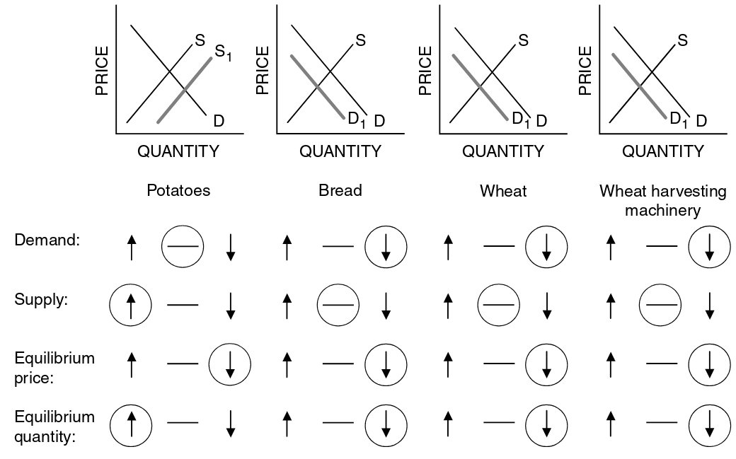
Source: Morton & Goodman (2003, p. 83)
TipSolution
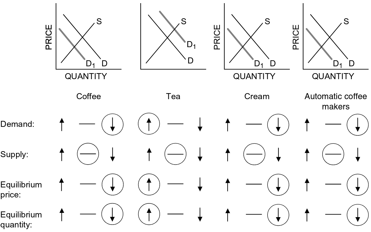
Source: Morton & Goodman (2003, p. 85)
Morton, J. S., & Goodman, R. J. B. (2003). Advanced placement economics: Teacher resource manual (3rd ed.). National Council for Economic Education.
Exercise 9.10 Supply and demand analysis
The diagram of Figure 9.9 shows the supply and demand schedule for a given good in a closed economy. The supply function is labeled with S and the demand function is labeled with D.
- What will be the equilibrium market price?
- How many items are traded?