22 Endowments

Learning objectives

Understand the expansion of the Ricardian trade model through the introduction of multiple production factors.
Learn that differences in countries’ factor endowments drive international trade patterns according to the Heckscher-Ohlin framework.
Understand that a country’s comparative abundance in a particular factor gives it a comparative advantage in goods that use that factor intensively.
Understand the tendency of international trade to equalize factor prices across countries.
Reflect on how trade can serve as a substitute for the physical mobility of production factors between countries.

Recommended reading: Suranovic (2012, Chapter 5)

Suranovic, S. (2012). International economics: Theory and policy (1.0 ed.). Saylor Foundation. https://open.umn.edu/opentextbooks/textbooks/276

22.1 Nobel prize winning theory

The theory which we discuss in this section explains trade because of different endowments. It is also known as the Heckscher-Ohlin model. It is named after two Swedish economist, Eli Heckscher (1879-1952) and Bertil Ohlin (1899-1979). Bertil Ohlin received the Nobel Prize in 1977 (together with James Meade). The HO-Model, as it is often abbreviated, was the main reason for the price. Here is an excerpt of the Award ceremony speech:

Your Majesties, Your Royal Highnesses, Ladies and Gentlemen,

The question why individuals, firms and nations exchange goods and services with each other, and how these processes are influenced by government policies, may be regarded as the basic issue in the science of economics. In the case of exchange between countries, the dominating theory was for a long time – from the beginning of the 19th century – David Ricardo’s theory of comparative advantage. Ricardo explained there the structure of foreign trade by differences in the production technology between nations. Over the years the theory was gradually improved upon in various ways, but a more basic overhaul did not take place until Bertil Ohlin in the early 1930’s published his work Interregional and International Trade, which is now a classic, and James Meade in the 1950’s came out with his important volumes on The Theory of International Economic Policy.

Bertil Ohlin showed in this work, which to some extent was inspired by a remarkable article by Eli Heckscher, that foreign trade may arise even if the production technology were identical in different nations. It is enough that the supplies of the factors of production of various kinds – such as labor of different types, capital, and land – differ among nations. The starting point of Ohlin’s theory is that a country tends to be an exporter of commodities that use relatively large amounts of the factors of production which are in ample supply as compared to domestic demand – in the hypothetical case without foreign trade. For instance, to take a simple example, if land is abundant in Australia while labor is relatively plentiful in England, we would expect Australia to be an exporter of commodities which for their production require much land, such as wool, while England would be an exporter of commodities the production of which requires relatively much labor, such as textiles.

From this simple theoretical structure, the so-called Heckscher-Ohlin model, follow a number of interesting theorems. One of them, the factor price equalization theorem, tells us that foreign trade tends to equalize the prices of the factors of production in different countries. For instance, when Australia starts to export land-intensive goods, the demand for land goes up relative to labor, with a rise in land prices as a result, while the export of labor-intensive goods by England pulls up wages there relative to the price of land. Thus, trade in commodities tends to have the same effects on the prices of the factors of production as if the factors themselves could move freely between countries. In this sense, commodity trade is a substitute for international mobility of the factors of production. Another inference from Ohlin’s theory is that a tariff on a labor-intensive good, such as textiles, affects the distribution of income in favor of labor in the importing country, while a tariff on a capital-intensive commodity, such as wool or steel, results in an income redistribution in favor of the owner of capital.

Source: www.nobelprize.org

The Ricardo model explains international trade as advantageous because of comparative advantages that are the result of technological differences. This means that comparative advantage in the Ricardian model is solely the result of productivity differences. The size of a country or the size of the countries’ endowments does not matter for comparative advantage in the Ricardian model because there is only one factor of production in Ricardian models, namely labor. However, the assumption that there is only one factor of production is unrealistic, and we should ask what happens if there is more than one factor of production but no productivity differences? What happens if the two factors are available differently in different countries? What is the significance of endowment differences for international trade? And which owner of a factor of production will be a winner when a country opens up to world trade, and who will lose? The HO model can provide answers to these questions.

In Table 22.1, I show that countries do indeed differ substantially in their total factor productivity, capital stock, and labor endowments, which are likely correlated with total population.

Table 22.1: Endowment differences across countries in 2010

RegionCode	Capital stock at current PPPs (in mil. 2011USD)	Population (in millions)	Capital stock per capita
ITA	10421041	60	174885
ESP	7806612	47	167518
FRA	10405968	65	160395
GBR	9973122	63	159019
DEU	12687682	80	157738
USA	48876336	310	157729
AUS	3332890	22	150382
CAN	5065392	34	148431
JPN	17161376	127	134790
SAU	3716382	28	132300
KOR	6052155	49	123287
TWN	2835890	23	122549
ROU	1271652	20	62647
VEN	1765996	29	60905
BRA	9869311	199	49691
RUS	6746460	143	47126
POL	1769004	39	45859
THA	2977965	67	44652
IRN	3234132	74	43555
ARG	1773984	41	43034
MEX	5054693	119	42613
TUR	2938288	72	40634
UKR	1616826	46	35420
IDN	8146254	242	33716
COL	1446480	46	31501
CHN	42218080	1341	31483
PER	681036	29	23185
PHL	1560017	93	16767
IRQ	443733	31	14375
IND	15356803	1231	12475

Source: Penn World Tables 9.0

22.2 The Heckscher-Ohlin (factor proportions) model

Assumptions:

Two countries: Home country and foreign country. Variables referring to foreign countries are marked with an asterisk, \(*\).
Two goods: \(x\) and \(y\).
Two factors of production: \(K\) and \(L\). This is new in relation to the Ricarkian model! Let’s name the factors \(K\) and \(L\), which stands for capital and labor.
Goods differ in terms of their need for factors of production: \[\frac{K_y}{L_y} \neq \frac{K_x}{L_x}.\] This means that one good must be produced in a capital-intensive way and the other in a labor-intensive way. If we assume that good \(y\) is capital intensive and good \(x\) is labor intensive in production, we can write: \[\begin{align*} \frac{K_y}{L_y} > \frac{K_x}{L_x}. \end{align*}\] In this inequality, the quantity of capital required to produce good \(y\), \(K_y\), is on the left-hand side relative to the quantity of labor required to produce good \(y\), \(L_y\), that is, the capital intensity of good \(y\).The capital intensity of good \(x\) is on the right-hand side of the inequality. Rewriting this inequality, we can express it in terms of labor intensities: \(\frac{L_y}{K_y} < \frac{L_x}{K_x}.\) It should be clear that both inequalities say the same thing.
No technology differences between countries: Since we already know from Ricardian theory that productivity or technology differences are a source of international trade, we do not want to explain the same thing again with the HO model. So we assume that all input coefficients are the same in all countries.
Different relative factor endowments: \[\frac{K}{L} \neq \frac{K^*}{L^*}.\] Since countries are assumed to have different factor endowments, the model links a country’s trade pattern to its endowment of factors of production. The capital-labor ratio in the home country, \(\frac{K}{L}\), must differ from the ratio abroad. Suppose the home country is capital-rich and the foreign country is labor-rich. Then we have the following ratios between capital and labor in the two countries: \[\begin{align*} \frac{K}{L} > \frac{K^*}{L^*}. \end{align*}\] This means that the capital-labor ratio (a country’s capital intensity) is higher in the home country than abroad. In terms of the ratio between labor and capital, that is, the labor intensity of a country, this can be expressed as follows: \(\frac{L}{K} < \frac{L^*}{K^*}.\) It should be clear that both inequalities say the same thing.
Free factor movement between sectors Both factors can be used in the production of both goods. Note that cross-country movement of factors (migration, foreign direct investment) is not allowed.
No trade costs Final products can be traded without any costs.
Equal tastes in countries and homothetic preferences Consumers in both countries have the same utility function. Homothetic preferences simply mean that for given relative prices, income does not affect the ratio of consumption.

22.3 Heckscher-Ohlin theorem

Consider that the home country has relatively more capital and the foreign country relatively more labor and that the good \(y\) is capital intensive in production whereas the good \(x\) is labor intensive.
Then it is relatively cheap for the home country to produce the capital-intensive good because it is endowed with a lot of capital, while it is relatively costly to produce the good with which the country is hardly endowed.
Thus, the home country has a comparative advantage in producing the capital-intensive good.
The opposite is true for the foreign country.

Heckscher-Ohlin Theorem

The capital abundant country exports the capital-intensive good. The labor abundant country exports the labor-intensive good.

In other words:

A country export goods that are intensive in its relatively abundant factor and will import goods that are intensive in its relatively scarce factor.

22.4 Factor-price equalization theorem

As a result of the Heckscher-Ohlin theorem, output of the good in which the country has a comparative advantage would increase. The capital intensive country will produce more capital intensive goods and the labor intensive country will produce more labor intensive goods.
As the production of the good that makes intensive use of the abundant resource increases, the demand for that resource will also increase. Demand for the scarce resource will also increase, but to a lesser extent.
If production of the good that intensively uses the scarce resource decreases, both abundant and scarce resources will be released, but relatively more of the scarce resource than of the abundant resource.
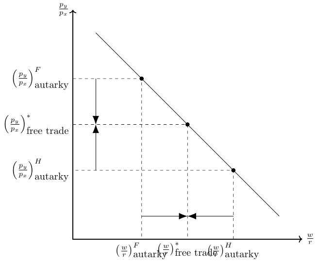
In autarky, the relatively scarce factor in the home country was labor and factor prices were as follows: \[ \frac{w}{r}>\frac{w^*}{r^*} \]
After opening to trade, production shifts to the home country so that the wage falls (\(w\downarrow\)) and the rent rises (\(r\uparrow\)).
After opening to trade, production shifts abroad so that the wage rises, \(w^*\uparrow\), and the rent falls, \(w^*\downarrow\).
This reallocation process, and hence the change in factor prices, continues until factor prices are equal in all countries: \[ \frac{w}{r}=\frac{w^*}{r^*} \]
Figure 22.1 visualizes the reasoning behind the factor-price equalization theorem.

Factor-price equalization theorem

The prices of the two factors of production (wage and rent) will be equalized across countries as a result of international trade in goods.

I recommend a clip of Mike Moore explaining how trade based on factor endowments affects wages and returns to capital, see this video:

Why does the Factor-Price Equalization Theorem not (fully) hold?

In the real world, factor prices do not equalize due to frictions such as transportation costs, trade barriers, and the presence of goods that are rarely or never traded.

Trade as an alternative to factor movements:

The factor price equalization theorem contains an interesting insight: if a country allows free trade in its products, it will automatically export the abundant factor indirectly in the form of goods that intensively use the abundant factor.

Exercise 22.1 Ricardo and Heckscher-Ohlin

Discuss the main differences of the Ricardian Model and the Heckscher-Ohlin Model.
Assume that only two countries, A and B, exist. Both countries are equally endowed with the only production factor labor which can be used to produce either good \(y\) or good \(x\). The table below gives input coefficients, \(a\), for both countries, that is, the units of labor needed to produce one unit of good \(y\) and good \(x\), respectively. Name the country with a comparative advantage in good \(y\).

	Countries
	A	B
Good \(y\)	10	11
Good \(x\)	1	2

Exercise 22.2 HO-Model in one figure

Suppose consumers from country A and the foreign country B like to consume two goods that are neither perfect substitutes nor perfect complements. Moreover, assume for simplicity that both countries have the same size but have different endowments, as stated in the assumptions above. Moreover, assume the factor intensity of production as stated in the assumptions above.

Sketch the production frontiers for both countries in autarky. Show graphically the relative price in autarky.
You will see that the relative prices of goods differ across countries: \[\begin{align*} \left(\frac{p_1}{p_2}\right)\neq\left(\frac{p_1}{p_2}\right)^*. \end{align*}\] That means, the Home country A has a comparative advantage in producing good \(1\).
Now, sketch the world market price that will maximize the utility.
Where are the new production and consumption points of both countries?
Show in the graphic how much each country trades.
I recommend a clip of Mike Moore who also explains the HO-Model with production possibility curves, see this video.

Solution

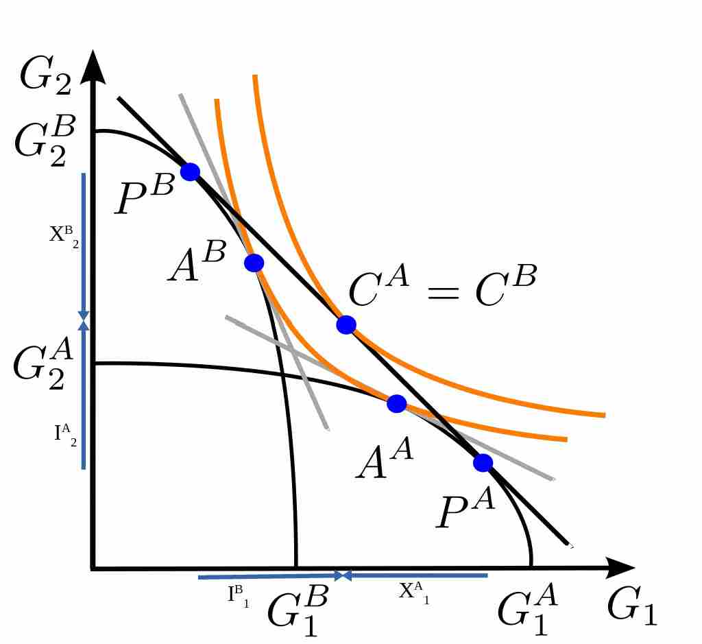
Two identical countries (A and B) have different initial factor endowments. I assume that country A is abundantly endowed with the production factor that is intensively used in the production of good 1, the reverse holds for country B. Thus, the two solid black lines in Figure 22.2 represents the respective production possibility frontier curves. The orange lines represents the respective indifference curves. Autarky equilibria are marked with \(A^{A}\) and \(A^{B}\), respectively. The production points in trade equilibrium are marked with \(P^A\) and \(P^B\), the consumption point of both countries is in \(C^A=C^B\). Thus, production and consumption points are divergent. The indifference curve under free trade is clearly above the other indifference curve in autarky. The solid black line that is tangient to the consumption point under free trade represents the utility maximizing world market price under free trade. The exports, \(X\), and imports; \(I\), are denotes correspondingly to the goods and country names.

Exercise 22.3 Multiple choice: HO-Model

Given are the assumptions of the Heckscher-Ohlin Model. In particular, assume that only two countries, A and B, and two goods, \(y\) and \(x\), exist. Consider the following data:

	Countries
	A	B
Factor Endowments
Labor Force	20	30
Capital Stock	30	40

If good \(y\) is capital intensive in production and good \(x\) is labor intensive in production then, following the Heckscher-Ohlin Theorem, …

country A will export good \(y\).
country B will export good \(y\).
both countries will export good \(y\).
trade will not occur between these two countries.

Solution

Multiple choice: HO-Model (Exercise 22.3)

Answer a) is correct.