13 Imperfect
Required readings: Emerson (2019, ch. 10 and 11),
Recommended readings: Anon (2020, ch. 6)
In earlier chapters, we looked at how free markets efficiently allocate resources. We stressed that this magic of the price system needs perfect markets to function. Although perfect competition isn’t found in reality, it’s a useful theoretical model. It helps us analyze markets and guide policymakers in dealing with market failures, where perfect market conditions aren’t met.
Sections Section 10.4 and Section 10.5 covered the welfare losses from price controls, taxes, and subsidies. Upcoming sections will come back to that and we will explore more sources of market failure, their effects, and how to counteract them.
It is important to note that, despite the absence of perfect market conditions in practice, centrally planned economies do not inherently outperform market-based systems. Historical experience suggests that a free-market-oriented capitalist approach is the most effective, albeit imperfect, system for economic organization.
Theory suggests that when firms make profits, new firms enter or existing firms expand. This increases supply, lowers prices, and eventually firms earn zero profit. At equilibrium, total revenue equals total cost, and firms don’t profit. Profits come from competitive advantages, which means firms aren’t price takers. This contradicts one of the assumptions of perfect competition. The most extreme competitive advantage is a monopoly, where one firm controls the entire supply and pricing of a good or service. We will discuss this further in the next section.
13.1 Theorems of welfare economics
There are two fundamental theorems of welfare economics. The first states that a market in equilibrium under perfect competition will be Pareto optimal in the sense that no further exchange would make one person better off without making another worse off. The requirements for perfect competition are as follows:
- There are no externalities and no transaction costs, and each actor has perfect information.
- Any efficient allocation of resources can be achieved through competitive markets, given the right redistribution of resources.
13.2 Types of imperfect market structures
To develop principles and make predictions about markets and how producers will behave in them, economists have developed numerous models of market structure, including the following:
- Monopolistic competition: also called competitive market, where there are a large number of firms, each having a small proportion of the market share and slightly differentiated products.
- Oligopoly: a market dominated by a small number of firms that together control the majority of the market share.
- Duopoly: a special case of an oligopoly with two firms.
- Monopsony: when there is only one buyer in a market.
- Monopoly: where there is only one provider of a product or service.
- Natural monopoly: a monopoly where economies of scale cause efficiency to increase continuously with the size of the firm. A firm is a natural monopoly if it can serve the entire market demand at a lower cost than any combination of two or more smaller, more specialized firms.
- Perfect competition: a theoretical market structure featuring no barriers to entry, an unlimited number of producers and consumers, and a perfectly elastic demand curve.
As one assumption of the perfect free market is that there is competition, it is evident that if there is just one or a few competitors, this assumption is not fulfilled. In the following, we discuss what happens to markets that don’t have perfect competition.
13.3 Price controls
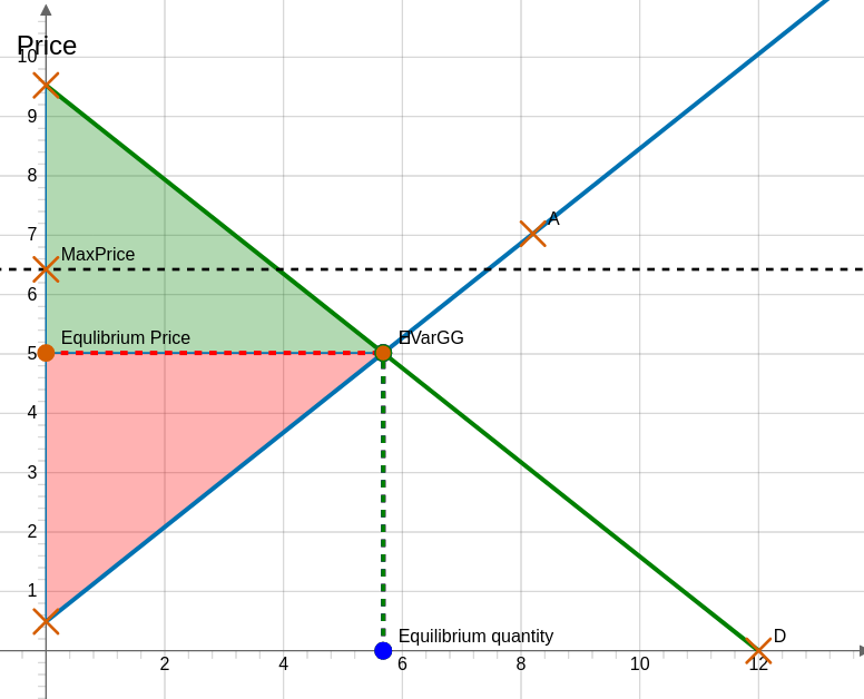
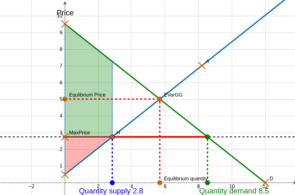
13.3.1 Maximum price
A legal maximum price, set to protect consumers, establishes an upper limit for the sale of a good. One example is price fixing in rental apartments. It is ineffective if set above the equilibrium price (see Figure 13.1); it becomes binding when placed below the equilibrium price (see Figure 13.2). This can lead to deadweight loss due to missed mutually beneficial transactions.
13.3.2 Minimum price
A legal minimum price is a rule that sets the lowest price for a product, protecting sellers. For example, minimum wage protects the seller of labor time. Only when this minimum price is higher than the normal price is it binding and affects the market.
13.3.3 Price controls
Analyze the two scenarios above. Can you sketch in both plots consumer and producer surplus? Who is better off? Who is worse off? And does overall welfare increase or decrease?
13.3.4 Taxes
Taxes change how things are bought and sold. When there’s a tax, people who buy things pay more, and people who sell things receive less money, no matter who the tax is on. Tax incidence shows how the burden of the tax is divided between buyers and sellers.
The tax has several effects:
- Quantity of goods sold decreases.
- Sales decrease after the tax is applied.
- The tax burden is shared between buyers and sellers, no matter who the tax is imposed on.
- There is a loss of welfare (deadweight loss).
Exercise 13.1 Tax consumer
Figure 13.3 illustrates the consequences of a fixed excise tax and its implied deadweight loss when the producers have to pay the tax (an excise tax is a tax imposed by the government that applies when a producer makes a sale. A fixed excise tax is an amount that the seller must return to the government for each unit sold to a customer).
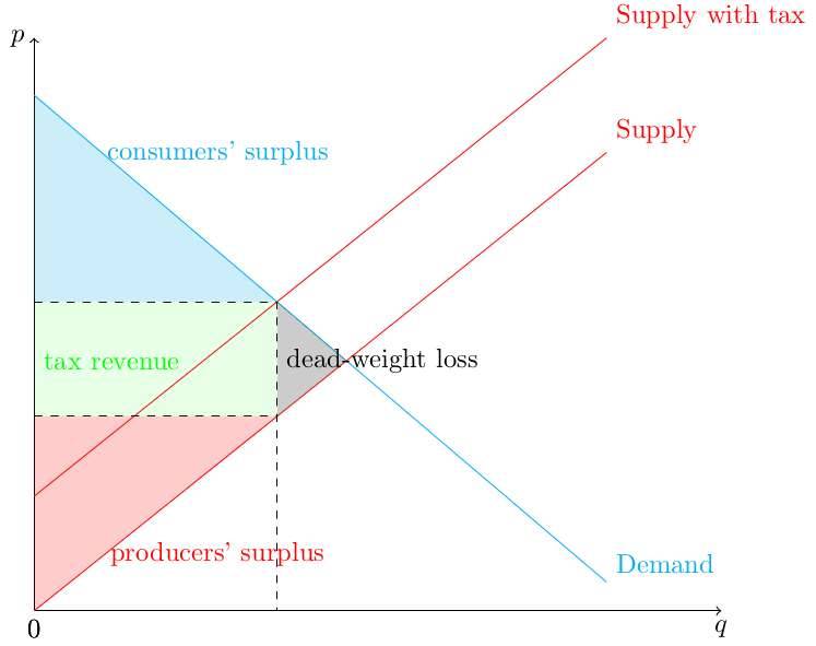
Sketch a similar figure: - When the consumer has to pay the tax. - When there is a price ceiling (a market where exchanges are not permitted above a certain price). - When there is a price floor (a market where exchanges are not permitted under a certain price).
Exercise 13.2 Laffer curve
The so-called Laffer curve is an economic concept that illustrates the relationship between tax rates and tax revenue. It is named after economist Arthur Laffer, who sketched the curve in 1974 on a napkin while talking to Dick Cheney and Donald Rumsfeld, two former important US politicians. The curve suggests that there exists a tax rate that maximizes government revenue. At very low and very high tax rates, the government revenue generated may be relatively low, as taxpayers either have little incentive to work (at very high rates) or can evade taxes (at very low rates).
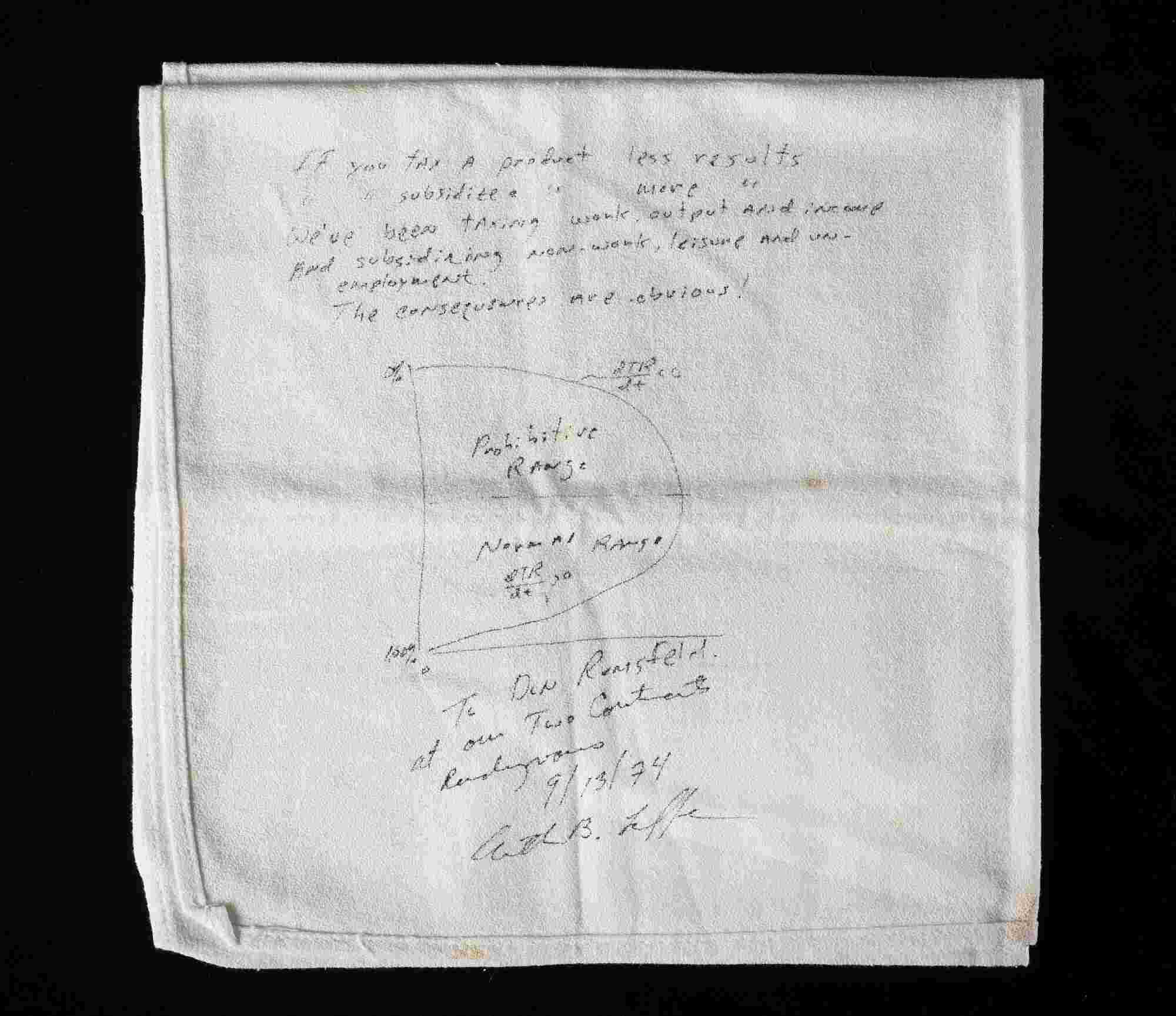
Source: National Museum of American History, see: Link.
Now, visit this interactive graph and consider the Laffer curve. What is the impact of the supply and demand elasticity? Can you always spot consumer surplus, producer surplus, tax revenue, and deadweight loss?
13.4 Subsidies
Subsidies are like negative taxes, producing the opposite impacts of taxes, which include:
- More quantity being bought and sold.
- A boost in total sales due to the subsidy.
- The benefits are shared between buyers and sellers, regardless of who receives the subsidy.
Exercise 13.5 Markets are connected
Read section Emerson (2019, ch. 11.1) and solve the following tasks.
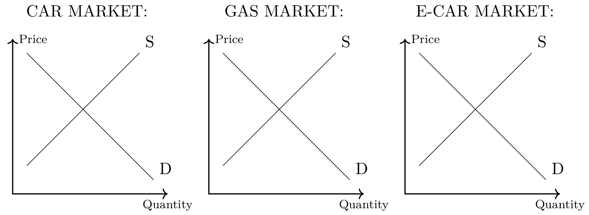
Consider the following goods: gasoline powered cars (cars), electricity powered cars (e-cars), and gasoline (gas).
- Are the goods cars and gas more likely to be substitutes or complements? Explain your decision.
- Indicate whether the following pairs of goods are more likely to be substitutes or complements: (1) cars and e-cars (2) e-cars and gas.
- Suppose a new, easily accessible, and large oil field is found. As a consequence, you expect that the price for gasoline will fall. Analyze the impact of this exogenous shock on the three markets in further detail. Assume that the price of gasoline does not alter the production of cars and e-cars.
The three plots in Figure 13.5 represent the three markets where the supply function \(S\) and demand functions $D $ refer to the market circumstances before the exogenous shock has happened.
Sketch in the three plots — for each market — shifts of the supply function and/or the demand function that may happen due to the exogenous shock. Discuss the new equilibrium prices and quantities in the respective markets.