24 Aggregate demand
Required readings: @Blanchard2013Blanchard.
Learning objectives:
Students will be able to:
- Understand that demand determines production in the short run.
- Recognize that increases in consumer confidence, investment demand, government spending, or decreases in taxes can increase equilibrium output in the short run.
- Learn how to derive the building blocks of our short-run model: the IS curve.
24.1 Stylized facts

24.2 How to fight an economic crisis

Source: Blanchard & Johnson (2013, p. 43)
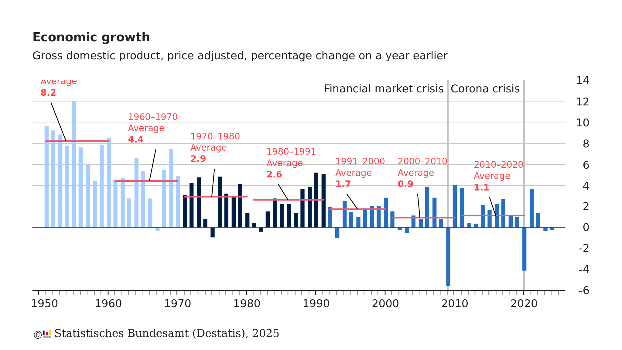
In times of economic crisis, people reduce their spending. Businesses cut back on orders and lay off workers, which further reduces consumption. This vicious cycle is illustrated in Figure 1. How can we break this cycle of reduced consumption and job loss? The answer is straightforward: boost aggregate demand. The upcoming section will elaborate and justify that answer further.
The coronavirus pandemic has slowed global commerce to a crawl. However, many large economies are taking significant actions to move through the crisis. How have national governments acted to lessen the economic impact of the pandemic?
To aid EU citizens, businesses, and countries in recovering from the COVID-19 economic downturn, EU leaders have developed a recovery plan for Europe. On 23 April 2020, they decided to establish an EU recovery fund to mitigate the crisis’s effects. By 21 July 2020, EU leaders approved a €1.824 trillion budget for 2021-2027. This package, which includes the Multiannual Financial Framework and Next Generation EU, will help rebuild post-pandemic and invest in green and digital transitions. Besides these measures, three safety nets totaling €540 billion are already in place to support workers, businesses, and countries. On 25 September 2020, the Council sanctioned €87.4 billion in financial aid to 16 member states via the EU’s emergency unemployment program, SURE.
The IMF Policy tracker summarizes the key economic responses governments are taking to limit the human and economic impact of the COVID-19 pandemic. The tracker includes 196 economies. See: IMF Policy Responses to COVID-19.
Germany’s federal government has adopted two supplementary budgets to tackle the COVID-19 crisis:
- €156 billion (4.9% of GDP) in March and €130 billion (4% of GDP) in June.
- They plan to issue €218.5 billion in debt this year to fund these initiatives.
Key measures include:
- Investments in healthcare equipment, hospital capacity, and vaccine research.
- Expanded access to short-term work subsidies (Kurzarbeit), childcare benefits for low-income parents, and basic income support for the self-employed.
- €50 billion in grants for small businesses and self-employed individuals affected by the pandemic, interest-free tax deferrals until year-end, and €2 billion in venture capital for startups.
- Extended unemployment insurance and parental leave benefits.
The June stimulus package offers temporary VAT reduction, income support for families, grants for struggling SMEs, local government financial aid, credit guarantees for exporters, and investments in green energy and digitalization. In August, the government extended short-term work benefits from 12 to 24 months.
At the same time, through the newly created economic stabilization fund WSF (Wirtschaftsstabilisierungsfonds) and the public development bank KfW (Kreditanstalt für Wiederaufbau), are increasing guarantee volumes and public guarantee access for various firms and institutions. Eligible entities may receive up to 100% in guarantees, raising the total by at least €757 billion (24% of GDP). These entities also facilitate public equity injections into strategically important firms.
In addition to the federal government’s fiscal package, many local governments (Länder and municipalities) have announced their own measures to support their economies, amounting to €141 billion in direct support and €63 billion in state-level loan guarantees.
24.3 Aggregate demand
When economists consider year-to-year shifts in economic activity, they focus on the interactions among production, income, and demand:
- Changes in the demand for goods lead to changes in production.
- Changes in production lead to changes in income.
- Changes in income lead to changes in the demand for goods.
24.3.1 The composition of GDP
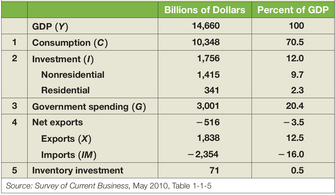
The GDP as a value-added measure can basically be subdivided into consumption, investment, government spending, and trade (see Figure 24.7).
24.3.1.1 Consumption, \(C\)
Consumption refers to the goods and services purchased by consumers, such as food, airline tickets, new cars, vacations, etc.
24.3.1.2 Investment, \(I\)
Investment is the purchase of capital goods. It includes nonresidential investment (e.g., firms buying new plants and machines) and residential investment (e.g., people buying new houses).
24.3.1.3 Government Spending, \(G\)
Government spending refers to the purchase of goods and services by federal, state, and local governments. It does not include government transfers (e.g., Medicare, Social Security) or interest payments on government debt. While these are government expenditures, they are not purchases of goods and services.
24.3.1.4 Imports, \(IM\)
Imports are the purchases of foreign goods and services by consumers, business firms, and the domestic government.
24.3.1.5 Exports, \(X\)
Exports are the sales of domestic goods and services to foreign countries.
24.3.2 Demand for goods
Denote the total demand for goods by \(Z\). Using the decomposition of GDP, we can write \(Z\) as \[ Z \equiv C + I + G + X - IM \] This equation is an identity (which is why it is written using the symbol \(\equiv\) rather than an equals sign). To think about the determinants of \(Z\) fruitfully, let’s make some simplifications to focus on the issue at hand:
- Assume that all firms produce the same good, which can then be used by consumers for consumption, by firms for investment, or by the government.
- A is an item that stands for both physical goods and services.
- Assume that firms are willing to supply any amount of the good at a given price level \(P\). This assumption allows us to focus on the role demand plays in the determination of output.
- Assume that the economy is closed, i.e., it does not trade with the rest of the world. Thus, both exports and imports are zero. Although this is untrue, this assumption simplifies our discussion because we won’t have to think about what determines exports and imports.
- Under the assumption that the economy is closed (a.k.a. in autarky), the demand for goods is simply the sum of (1) consumption, (2) investment, and (3) government spending:
\[ Z \equiv C + I + G \]
(1) Consumption
\[ C = C(\underbrace{Y_D}_{(+)}) \]
The consumption function, \(C = C(Y_D)\), captures how consumer spending changes with disposable income. The \((+)\) indicates that consumption increases as disposable income (\(Y_D\)) rises, though not one-to-one. Disposable income is what remains after taxes (\(T\)) and government transfers:
\[ Y_D \equiv Y - T \]
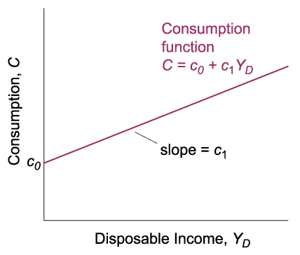
A linear version of the consumption function is shown in Figure 24.8:
\[ C = c_0 + c_1 Y_D \]
- This function has two parameters, \(c_0\) and \(c_1\):
- \(c_0\) is the function’s intercept.
- \(c_1\) is the marginal propensity to consume, showing the effect of an additional dollar of disposable income on consumption \((0 \leq c_1 < 1)\).
Source: Blanchard & Johnson (2013, p. 47)
(2) Investment
Variables within the model can be endogenous, meaning they depend on other variables in the model. Conversely, exogenous variables are those not explained within the model. Here, we treat investment as given, making it exogenous. For now, we write:
\[ I = \bar{I} \]
(3) Government spending
Government spending (\(G\)) and taxes (\(T\)) represent fiscal policy, which involves the government’s decisions on taxation and spending. We treat \(G\) and \(T\) as exogenous variables because they are typically set by the government, and we won’t explain them further in the model. As this assumption remains unchanged, we don’t use a bar notation for \(G\) and \(T\), simplifying the notation. Note that \(T\) refers to taxes minus government transfers.
24.3.3 Equilibrium in the goods market
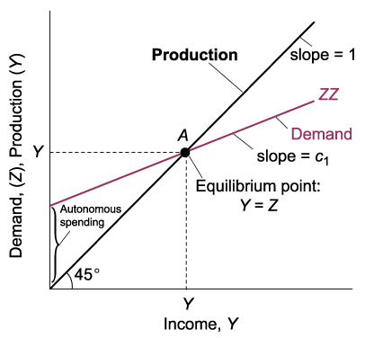
Equilibrium output is determined by the condition that supply (output/production) be equal to demand.
24.3.3.1 The determination of equilibrium output
Equilibrium in the goods market occurs when production (\(Y\)) equals the demand for goods (\(Z\)).
\[ Y = Z \]
If you’re unfamiliar with the term equilibrium, you can find more information here.
Then, using our assumptions of (1) to (3):
\[\begin{align*} Y &= \underbrace{C + I + G}_Z \\ Y &= \underbrace{c_0 + c_1 Y_D}_{C} + \underbrace{\bar{I}}_I + G \\ Y &= c_0 + c_1 \underbrace{(Y - T)}_{Y_D} + \bar{I} + G \\ \end{align*}\]
The equilibrium condition requires production (\(Y\)) to equal demand (\(Z\)). Demand, \(Z\), depends on income, \(Y\), which in turn is equal to production. We use \(Y\) to denote both because GDP can be viewed from the production side or the income side.
Once the model is built, we solve it to understand what influences output levels, like changes in government spending. Solving the model involves not only algebra but also understanding the reasons behind the results. We use graphs to visualize the results—sometimes skipping algebra—and words to describe the outcomes and underlying mechanisms.
Economists employ these three tools to solve a model effectively:
- Algebra: Ensures logical consistency.
- Graphs: Aids in building intuitive understanding.
- Words: Provides clarity and explanation.
24.4 The model using algebra
Let’s derive key components from the equilibrium equation \(Y = c_0 + c_1(Y - T) + \bar{I} + G\) to \(Y\):
\[ Y = \underbrace{\frac{1}{1 - c_1}}_{\text{multiplier}} \underbrace{\left(c_0 + \bar{I} + G - c_1 T\right)}_{\text{autonomous spending}} \]
Components:
- Autonomous Spending: Independent of output since all variables are exogenous.
- The Multiplier: Greater than one because the propensity to consume \((c_1)\) ranges between zero and one. As \((c_1)\) approaches one, the multiplier grows. An increase by one unit in autonomous spending raises output by more than one unit.
24.5 FAQ
Where does the multiplier effect come from?
- From the consumption equation, an increase in \(c_0\) boosts demand. This prompts higher production, which raises income. The rise in income further boosts consumption and demand, creating a cycle.
- The initial demand increase triggers successive output increments. Each production increase elevates income and demand again—continuing the cycle.
- The multiplier sums the successive production increases stemming from a demand rise.
- When demand grows by $1 billion, production rise after \(n\) rounds equals $1 billion times:
\[ 1 + c_1 + c_1^2 + \dots + c_1^n = \frac{1}{1-c_1} \]
This is a geometric series. If you feel like you need explanations to that, please consider Appendix B.
Is the government omnipotent?
- Adjusting government spending or taxes can be challenging.
- Predicting the responses of consumption and investment is uncertain.
- Expectations significantly influence outcomes.
- The pursuit of specific output levels might lead to negative consequences.
- Budget deficits and public debt could have long-term effects.
How long does it take for output to adjust?
- Output increases gradually in response to heightened consumer spending, not immediately reaching the new equilibrium. This depends on firms revising production schedules.
- Understanding the timeline for output adjustment is known as the dynamics of adjustment.
What is the value of the multiplier in the real world?
To determine the multiplier’s value and examine behavioral equations, economists use econometrics, involving statistical methods. The process is complex, with varying results based on conditions.
Ramey (2019) observes effects of spending during the financial crisis:
Reviewing the estimates, I come to the surprising conclusion that the bulk of the estimates for average spending and tax change multipliers lie in a fairly narrow range, 0.6 to 1 for spending multipliers and -2 to -3 for tax change multipliers. However, I identify economic circumstances in which multipliers lie outside those ranges.
24.6 The model using graphs
Source: Blanchard & Johnson (2013, p. 51)
Source: Blanchard & Johnson (2013, p. 52)
24.7 The model using words
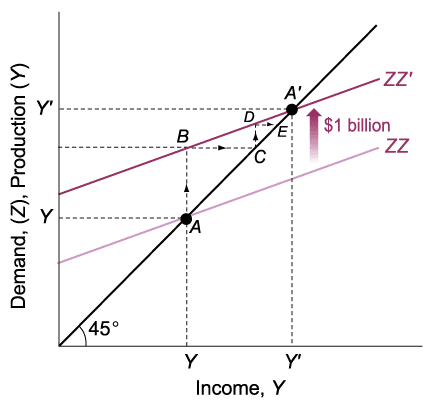
- The first-round demand increase leads to an equal production rise of $1 billion, shown by the distance AB.
- This production increase results in an equal income rise, indicated by the distance BC, also $1 billion.
- The second-round demand increase, shown by distance CD, equals $1 billion (the first-round income rise) times the propensity to consume, \(c_1\) — resulting in $\(c_1\) billion.
- This second-round demand increase induces an equal production rise, shown by distance CD, and consequently an equal income rise, indicated by distance DE.
- The third-round demand increase results in $\(c_1\) billion (second-round income increase) times \(c_1\), the marginal propensity to consume; equaling $\(c_1 \cdot c_1 = c_1^2\) billion, and so forth.
- An increase in autonomous spending has a greater than one-for-one effect on equilibrium output.
- An increase in demand leads to higher production and corresponding income growth. Consequently, output increases are larger than the initial demand shift, multiplied by the multiplier.
24.7.1 The goods market and the investment-savings (IS) relation
Recall: Equilibrium in the goods market exists when production, Y, equals demand for goods, Z. In the simple model above, the interest rate did not affect goods demand. The equilibrium condition was:
\[Y = C(Y-T) + I + G\]
24.7.2 The derivation of the IS curve
Now, let us loosen the assumption that investments are exogenous by capturing the effects of two determinants of investment:
- The level of sales, \(Y\), is positively associated with investments \(\left(\frac{\partial I}{\partial Y}>0\right)\)
- The interest rate, \(i\), is negatively associated with investments \(\left(\frac{\partial I}{\partial i}<0\right)\)
\[I = I(Y, i)\]
Considering the above investment relation, the equilibrium condition in the goods market becomes:
\[Y = C(Y-T) + I(Y, i) + G\]
The derivation of the IS curve is visualized in Figure 24.11.
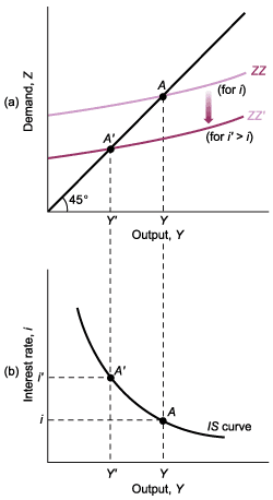
Source: Blanchard & Johnson (2013, p. 88)
24.7.3 Shifts of the IS curve
G, I and T can shift the IS curve. For example, an increase in taxes shifts the IS curve to the left.
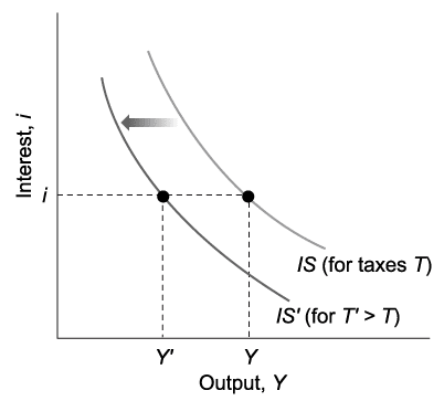
Source: Blanchard & Johnson (2013, p. 89)
24.8 Investment equals savings
Savings is the sum of private plus public savings.
Private saving (\(S\)) is saving by consumers:
\[ S \equiv Y - T - C \]
Public saving equals taxes minus government spending:
- If \(T > G\), the government has a budget surplus—public saving is positive.
- If \(T < G\), the government has a budget deficit—public saving is negative.
\[\begin{align*} Y &= C + I + G \\ \Rightarrow \underbrace{Y - T - C}_S &= I + G - T \\ \Rightarrow S &= I + G - T \\ \Rightarrow I &= \underbrace{S}_{\text{private savings}} + \underbrace{(T-G)}_{\text{public savings}} \end{align*}\]
- Thus, if \(T = G\), then \(I = S\).
- The equation above states that equilibrium in the goods market requires that investment equals saving—the sum of private plus public saving.
- This equilibrium condition for the goods market is called the IS relation.
- IS stands for investments equals savings.
- What firms want to invest must be equal to what people and the government want to save.
24.9 Summary
What you should remember about the components of GDP:
- GDP is the sum of consumption, investment, government spending, inventory investment, and exports minus imports.
- Consumption (\(C\)) is the purchase of goods and services by consumers. It’s the largest component of demand.
- Investment (\(I\)) includes nonresidential investment—buying new plants and machines by firms—and residential investment—buying new houses or apartments by individuals.
- Government spending (\(G\)) refers to goods and services purchased by federal, state, and local governments.
- Exports (\(X\)) are goods purchased by foreigners.
- Imports (\(Im\)) are goods purchased by U.S. consumers, firms, and government from abroad.
- Inventory investment is the difference between production and purchases, which can be positive or negative.
What you should remember about our first model of output determination:
- In the short run, demand determines production. Production equals income, which in turn affects demand.
- The consumption function depicts consumption dependence on disposable income, with the propensity to consume showing how much consumption rises for a given increase in disposable income.
- Equilibrium output is the output level where production matches demand. In equilibrium, output equals autonomous spending multiplied by the multiplier. Autonomous spending is demand that doesn’t depend on income, and the multiplier is \(\frac{1}{1-c_1}\), where \(c_1\) is the propensity to consume.
- Increased consumer confidence, investment demand, government spending, or lowered taxes all boost equilibrium output in the short run.