22 Long-run growth
Required readings:
Blanchard & Johnson (2013, ch. 11)
Recommended readings:
Blanchard & Johnson (2013, ch. 10-12) and Romer (2006, pp. 5–29)
Learning objectives:
Students will be able to:
- Understand how capital accumulates over time and its implications for economic growth.
- Analyze the impact of the diminishing marginal product of capital on differing growth rates across countries.
- Describe the principle of transition dynamics, where countries farther below their steady state experience faster growth.
- Identify the limitations of capital accumulation and recognize areas of economic growth that remain unexplained.
22.1 Preface
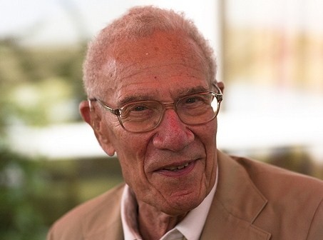
This chapter focuses on the determinants of economic growth in the long run. We present a growth model developed independently by Solow (1956) and Swan (1956) known as the Solow-Swan growth model, the neoclassical growth model, or simply the Solow model. Robert Solow (see Figure 22.1) received in 1987 Nobel Memorial Prize in Economic Sciences for his contributions.
Long run refers to long-term trajectories spanning decades, not cyclical movements. These models consider real income or real output and disregard factors significant in the short run, like inflation or demand.
22.2 Stylized facts
22.2.1 Hockey-stick growth
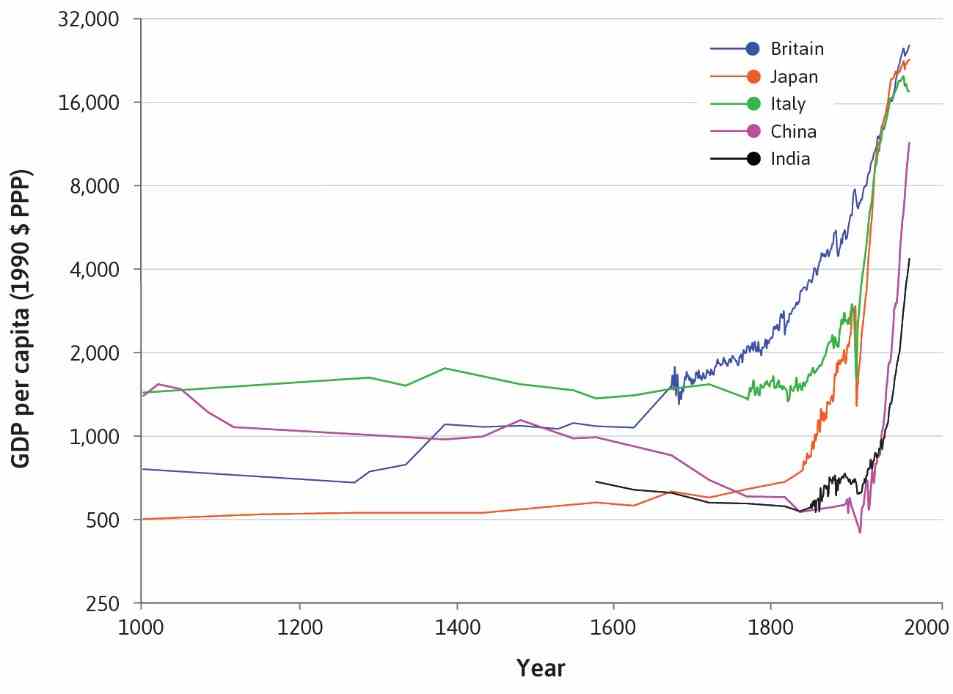
In Figure 22.3, it’s evident that numerous countries have witnessed a form of hockey-stick growth. Growth take-off occurred at different points in time for various countries: Britain was the first country to experience sustained economic growth, starting around 1650. In Japan, it occurred around 1870. The kink for China and India happened in the second half of the 20th century. Some economies only saw substantial improvements in living standards after gaining independence from colonial rule.
The Industrial Revolution, also called the Technological Revolution, was a transformative era from the late 18th to 19th centuries. It introduced advances, like machinery and steam power, that transformed manufacturing and led to urbanization, reshaping economies, labor, and society.
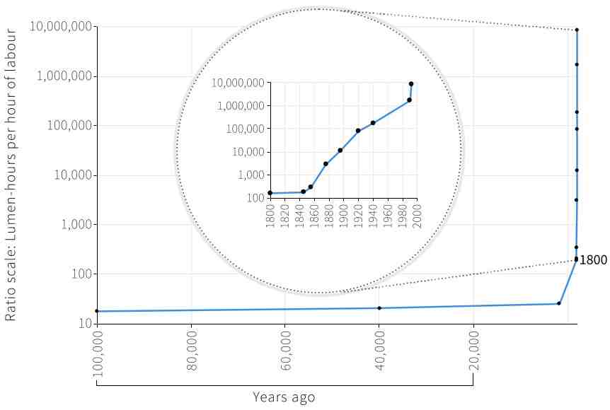
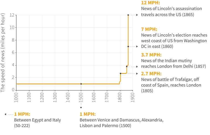
Technology is the process that uses inputs to produce outputs. For example, a cake recipe outlines the combination of inputs (e.g., flour, energy) and activities (e.g., stirring) needed to make the cake. Technological changes significantly reduced work time needed in production, allowing increased living standards. Figures Figure 22.4, Figure 22.5, and Figure 22.6 demonstrate rapid technological advancements impacting welfare.
Source: CORE Econ (2025)
Source: CORE Econ (2025)
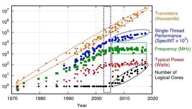
Source: Rusanovsky et al. (2019)
22.2.2 Population
Population growth displays a hockey-stick pattern, as shown in Figure 22.7. The figure illustrates the link between economic development and population growth. Although growth is slowing due to changing demographics, with birth rates falling faster than death rates, an annual growth rate of 1% still results in the world population doubling roughly every 70 years.
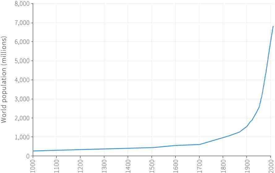
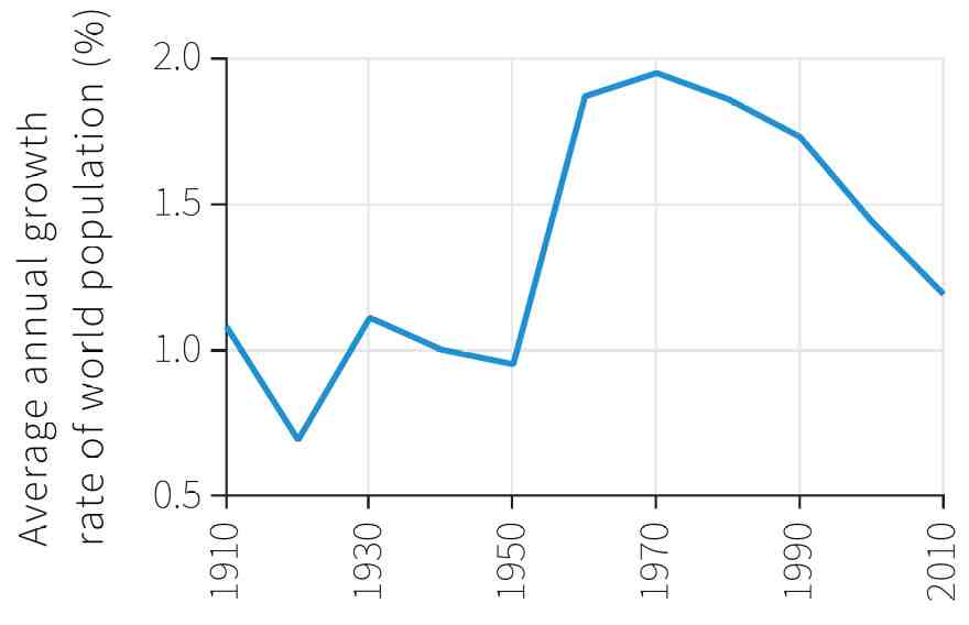
Source: CORE Econ (2025)
22.2.3 Fluctuations
Figure 22.8 illustrates long-term GDP growth in the UK, highlighting fluctuations and severe crises.
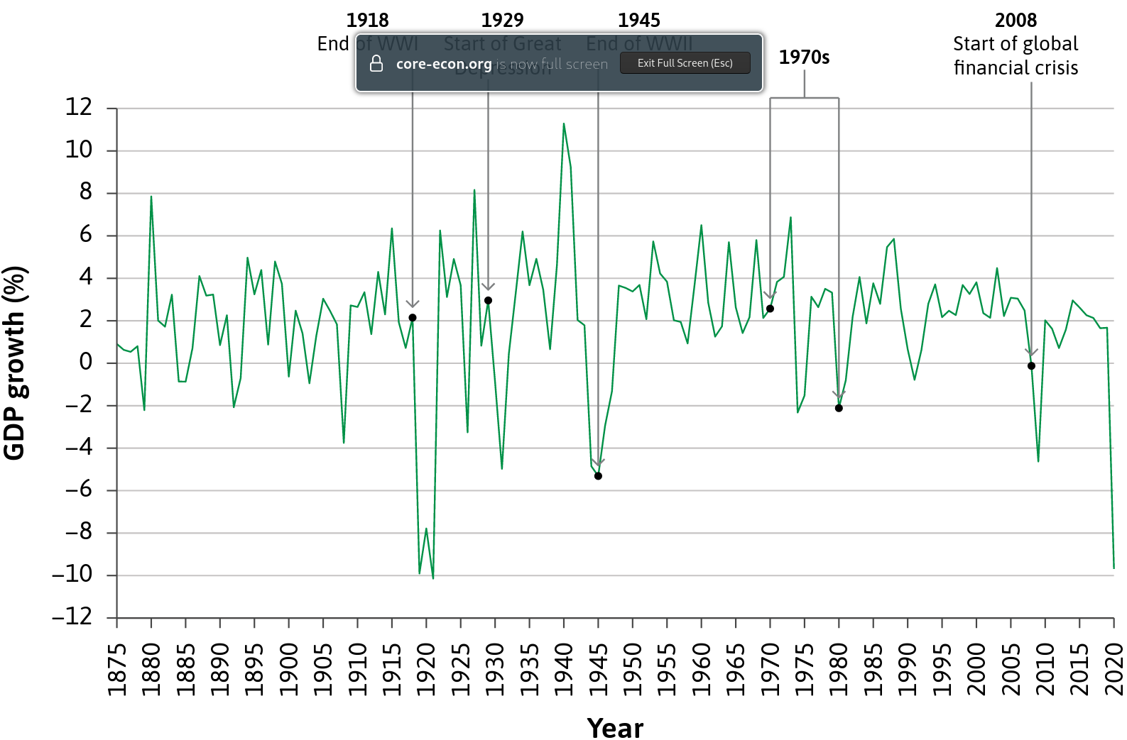
Source: www.core-econ.org
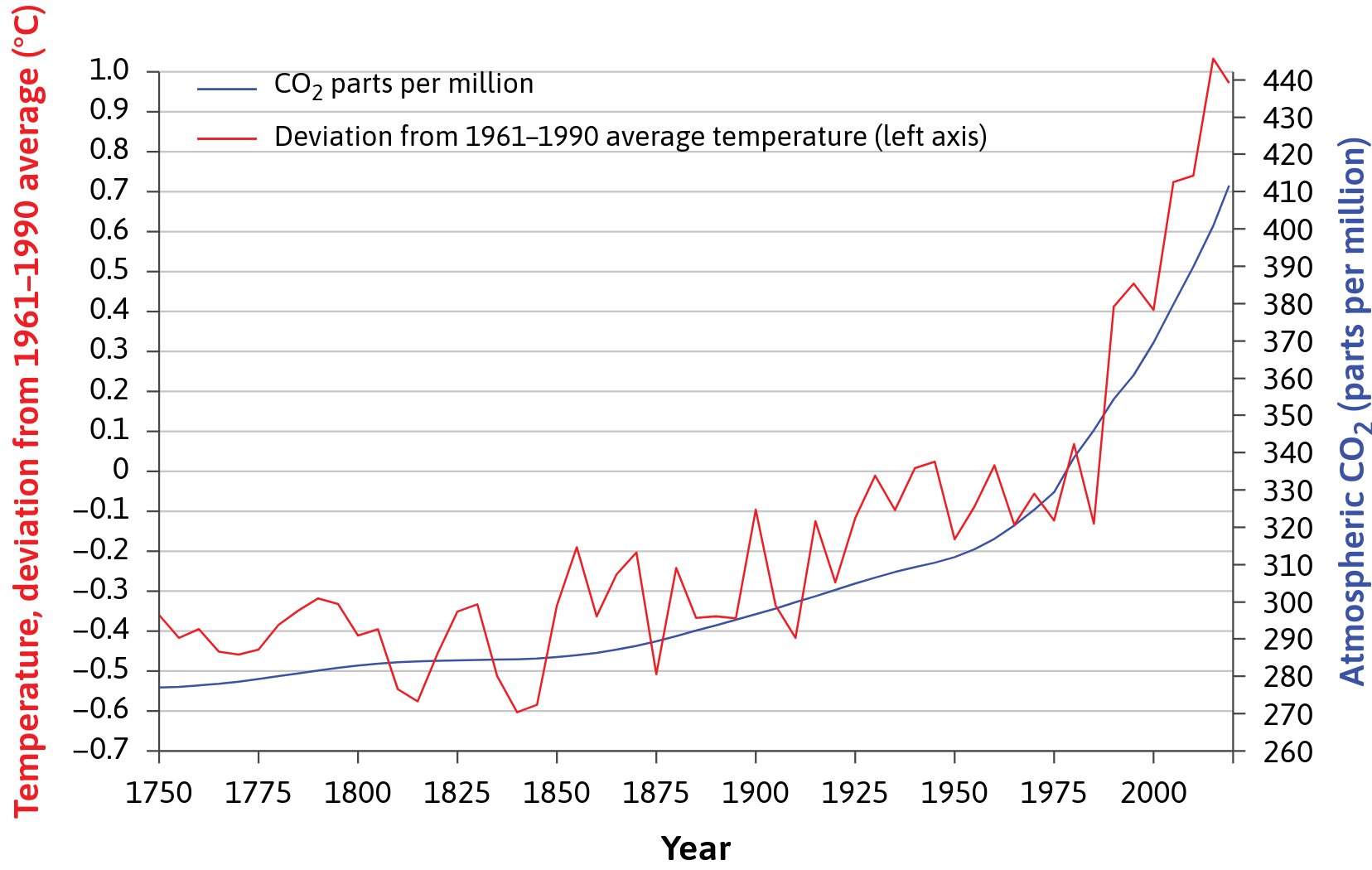
22.2.4 Nature
Environmental consequences arise from increased production and population growth, impacting global climate change and local pollution, deforestation. New technologies may offer potential solutions. Figure 22.9 illustrates significant environmental measures.
Source: www.core-econ.org
22.3 Solow model
22.3.1 Introduction
Source: Youtube
The nicely animated video of Figure 22.10 discusses unexpected economic growth situations and presents two puzzles: Germany and Japan’s rapid growth after World War II despite heavy losses, and China’s astonishing growth compared to advanced economies which have better institutions and more capital. The Solow Model of Economic Growth is introduced to help understand these dynamics and distinguish between “catching up” and “cutting-edge” growth. The model simplifies growth factors: labor (\(L\)), human capital (\(L\cdot e\)), physical capital (\(K\)), and ideas (\(A\)). These inputs work together in a production function to generate output. The abstraction of the production function will be further simplified in upcoming videos, starting with an exploration of how capital contributes to economic growth.
Here is a transcript of the video:
Here’s a fact about economic growth that might seem counterintuitive. During World War II, Germany and Japan suffered heavy losses. Millions of people were killed. Entire cities were flattened. Roads, bridges, factories, and other resources critical to an economy were destroyed. Yet, following World War II, Germany and Japan both grew quickly. In fact, they grew much faster than did the United States. Many people wondered what was going on. Why were the losers of the war growing faster than the winners? Here’s another puzzle. In the past several decades, China has been growing at astonishing rates of growth – 7 to 10% per year. Remember, at those rates, the standard of living – it’s doubling every 7 to 10 years. In contrast, in the advanced economies, like the United States, Canada, or France, they’re growing around 2% per year, doubling only once every 35 years. So here’s the puzzle. In the previous talks, we said that the way to get a high standard of living and economic growth is to have good institutions, like property rights, honest government, political stability, a dependable legal system, and competitive and open markets. But in each one of these cases, there’s no question that the advanced economies have better institutions than does China. Plus, the advanced economies – they’ve got more human and physical capital. So if the advanced economies have got better institutions and more capital, why are they growing slower than China? To solve these puzzles, we’re going to be drawing on an important economic model: the Solow Model of Economic Growth, named for Robert Solow, who won the Nobel Prize. The Solow Model will help us to better understand the dynamics of growth. The Solow Model is also going to help us to draw a distinction between two types of growth: catching-up growth and cutting-edge growth. As we’ll see, catching up can be much faster than growing on the cutting edge. Now, you might ask, “What’s an economic model?” An economic model is a simplified framework that helps us to understand a more complex reality. We’re going to be using a super simple version of the Solow Model that boils economic growth down to just a few key variables and some basic mathematics. Now, although it’s simple, the Solow Model can provide us with some deep insights into the causes of growth. A key part of the model is a production function – a simplified description of how resources, inputs, are used to produce output. So let’s take a look at some of the inputs into our production function. The first key input is us, people. We use the letter\(L\)to represent labor. The more educated people are, the more effective their labor. So we can multiply\(L\)by\(e\)for education. Together, these two variables represent human capital. Next is physical capital, represented by the letter\(K\).\(K\)is all of our factories, and tools, and so forth. Last, but certainly not least, is ideas, represented by the letter\(A\).\(A\)represents all of our knowledge about how to combine capital and labor to produce valuable output. Everything from how to transport stuff without carrying it on your back, to how to keep diseases from spreading, to how to add up numbers in a fraction of a second.\(A\)is ideas, and better ideas mean that we can get more bang for our buck, more output from the same inputs of capital and labor. We can think of human capital, physical capital, and ideas being used together to produce output. That’s the idea of our production function. Now, right now our production function is very abstract. But in future videos, we’re going to boil it down even more and make our production function concrete. We’re going to start in the next video by taking a closer look at how capital – machines, factories, roads, and so forth – how capital contributes to economic growth. Let’s dig in.
22.3.2 Steady state
Source: Youtube
Study the video of Figure 22.11 and the transcript of the video:
Let’s continue our exploration of the Solow Growth Model. In our last video, we covered how physical capital faces the iron logic of diminishing returns. Now let’s turn to another unfortunate aspect of physical capital: capital rusts. Roads get potholes and need to be repaired, tools wear out, trucks break down. In short, we say that capital depreciates. Now let’s put the amount of capital on the horizontal axis and the amount of depreciation on the vertical axis. We can then model the relationship like this. Depreciation increases at a constant rate as the capital stock increases. The more capital you have, the more capital depreciation you have. Now let’s add a new aspect to our model. Where does the money for capital accumulation come from? From savings and investment. When we create economic output, we can either consume it or save it. What we don’t consume can be saved and invested in new capital. So suppose we invest a constant fraction of our output. Let’s say we devote 30% of output to investment. We can now add an investment curve to our graph. It’ll mimic the shape of the output line since investment is just a constant fraction of output. Notice that our first units of capital – they’re very productive and so they create a lot of output and thus also a lot of investment. But as we add more and more units of capital, we get less output and also less investment. That’s the iron logic of diminishing returns once again. Now let’s put investment and depreciation on the same graph. Depreciation is growing at the same rate as the capital stock grows. Each new unit of capital creates an equal amount of depreciation. Now notice that when investment is greater than depreciation, that means the capital stock must be growing. We’re adding more units of capital than are depreciating. But as the capital stock grows – investment and depreciation – they’re on a crash course to intersect. When this happens, we’ve reached what is called the Steady-State Level of Capital. The steady-state is the key to understanding the Solow Model. At the steady-state, investment is equal to depreciation. That means that all of investment is being used just to repair and replace the existing capital stock. No new capital is being created. Now remember, we’ve assumed that all the other variables in the model – they’re not changing. So if the capital stock isn’t growing, nothing is growing. In other words, when we reach the Steady-State Level of Capital we’ve also reached the Steady-State Level of Output. Now suppose you ended up on the other side of the steady-state point – over here. You’d find that depreciation is greater than investment. That means some of the capital stock needs repair, but there isn’t enough investment to do all of the needed repairs, so the capital stock shrinks, pushing you back towards the steady state. So to the left of the steady-state we have investment greater than depreciation and the capital stock is growing. To the right of the steady-state we have the opposite – depreciation is greater than investment, and the capital stock – it’s shrinking. Either way, we always end up moving towards the steady-state. Let’s go back to our earlier example of Germany after the end of World War II. Since the capital stock is low, it’s also very productive and we get a lot of output from the first new roads and factories after the war. We’ve already mentioned that point. But in addition, we now see that when the capital stock is very productive and producing a lot of output, we will also be producing a lot of investment. So in the next period the capital stock will be even bigger than before and we’ll get even more output. Plus, since the capital stock is low, we don’t have much depreciation to take care of. So with the investment, it will mostly be generating new capital, not replacing old capital. Now over time, however, both of these forces - they weaken. The returns to capital diminish and depreciation eats up more and more of investment. A country with a lot of roads, and bridges and factories - it’s doing well, but it also has to invest a lot just to maintain all those roads and bridges and factories. And this is exactly what we saw in Germany and Japan after World War II. Growth rates started out very high, but as those countries caught up, growth rates declined. Now perhaps our friend\(K\)still has one more trick up his sleeve to get the economy growing. What if we started to save more of our output? A higher savings rate shifts the investment curve up like this. Now investment is higher than depreciation, so we’re adding to the capital stock and the economy is back to growing. However, you can see that the same dynamic exists as before. The iron logic of diminishing returns means that we’ll again end up at a new steady-state level of capital. The higher savings rate - it spurs growth for a time and it does increase the steady-state level of output. But, at the new steady-state, investment once again equals depreciation and we get zero economic growth. Accumulation of physical capital can only generate temporary growth. In our next video, we’ll take a look at how human capital influences growth.
22.3.3 Technological progress
Source: Youtube
Study the video of Figure 22.12 and the transcript of the video:
We’ve covered a lot of the super simple Solow Model. We’ve looked at the dynamics of capital accumulation, how changes in savings rates influence growth, and we’ve looked at some of the predictions of the Solow Model. One thing we’ve learned is that the model seems to inevitably predict that we end up in a steady state with no growth. Now, however, we’re going to turn to the last of our variables: ideas. Can ideas keep us growing? Better ideas mean that we get more bang for our buck, more output from the same inputs of capital and labor. Alternatively, we can think about this as increasing our productivity. Henry Ford, for example, took ideas from lots of other industries, like meatpacking, bicycle making, and brewing, and he combined them in a way that had never before been used in the manufacturing of automobiles. This novel combination of ideas sparked a dramatic increase in productivity that transformed the world. The same types of processes – they’re continuing today, and in all industries, increasing output per worker across the economies. So let’s go back to our previous graph of capital and output. We can now add ideas as a multiplier. Better ideas multiply the output from the same capital stock. So, if A increases from 1 to 2, that’s a doubling of our productivity. And that shifts the output curve up. When output doubles, so does investment. Now, once again, investment is greater than depreciation. So we begin accumulating capital once again. And that further boosts our output. So better ideas spur more output, which creates more investment, which leads to capital accumulation. So better ideas lead to growth in two ways: the increased productivity of a given capital stock, and the increased investment, which increases capital accumulation. Now imagine that ideas are constantly improving. You’d have continual shifts upward of the output curve. And that means continual shifts upward of the investment curve. We’d always stay to the left of the steady state, and there, we’d continually grow. So growth at the cutting edge – it’s determined by how fast new ideas are formed, and how much those new ideas increase our productivity. So that’s our super simple Solow Model. It combines a model of catching up growth due to capital accumulation, with a model of cutting-edge growth due to idea accumulation._
22.3.4 Solow’s central question
Question: Can capital accumulation lead to long-term growth and perpetual improvements in living standards? Formally speaking, can the following circular relationship last forever and lead to sustainable growth in production: \[Y \uparrow \rightarrow S \uparrow \rightarrow I \uparrow \rightarrow K \uparrow \rightarrow Y \uparrow \dots\]
Robert M. Solow’s answer is: No, capital accumulation can boost growth only for some time. The only long-term key to growth is technological progress.
In the 1950s, the Soviet Union launched a growth offensive with extremely high investments, primarily in heavy industry. The idea was to spur growth through the accumulation of capital. Howver, history was not really on their side as far as we can judge that. Here is a popular quote from Soviet First Secretary Nikita Khrushchev while addressing Western ambassadors at a reception at the Polish embassy in Moscow on November 18, 1956 (Time Magazine, 1956).
“Whether you like it or not, history is on our side. We will bury you!”
22.4 The formal Solow model
There are many different versions of the Solow model. Each has its unique way of writing things down, which might puzzle newcomers trying to understand it.
To make your reading of research easier, let me introduce you to the approach taken by (Romer, 2006, pp. 5–29). In his widely-recognized book for graduate students, he presents the classic form of the model. Despite its challenging aspects, it’s designed to be quite comprehensible.
22.4.1 Production
The heart of any theory of growth is a production function (PF) as it describes how output is made from different factors of production. Production in the Solow model takes the form:
\[Y(t) = f(K(t), A(t)L(t))\]
where \(Y\) is output, \(K\) is the input of physical capital (buildings and machines), \(L\)is the input of labor, and \(A\) is knowledge or the effectiveness of labor. Time\(t\)does not enter production directly but only through \(A\), \(K\), and \(L\). As \(A\) and \(L\) enter multiplicatively, \(AL\) is usually interpreted jointly as effective labor.
For convenience, the time argument (\(t\)) will be dropped, and the PF can be rewritten:
\[ Y = f(K, AL) \]
22.4.2 Constant returns to scale
If output changes by the factor \(c\) when every production factor is multiplied by \(c\), then the production function has constant returns to scale (CRS). Production in the Solow model is assumed to take place at constant returns to scale:
\[ f(c \cdot K, c \cdot AL) = c \cdot f(K, AL) \qquad \text{for all } c \geq 0 \]
22.4.3 Intensive form
CRS allows us to work with the PF in intensive form. Setting \(c\) to be \(\frac{1}{AL}\):
\[\begin{align} f\left(\frac{1}{AL} \cdot K, \frac{1}{AL} \cdot AL\right) &= \frac{1}{AL} \cdot \underbrace{f(K, AL)}_{Y}\\ \Leftrightarrow f\left(\underbrace{\frac{K}{AL}}_k, 1\right) &= \underbrace{\frac{Y}{AL}}_y\\ f(k) &= y \end{align}\]
where \(k\) is defined as \(\frac{K}{AL}\) and denotes the amount of capital per unit of effective labor, and \(y\) is defined as \(\frac{Y}{AL}\) and denotes the output per unit of effective labor.
22.4.4 Inada conditions
The intensive form production function (PF) is assumed to satisfy the following conditions: \[\begin{align*} f(0) &= 0,\\ f'(k) &> 0,\\ f''(k) &< 0. \end{align*}\]
A PF satisfying these assumptions is shown in panel a) of Figure 22.13. A nice series of lecture units explaining the Solow model can be found here.
22.4.5 Cobb-Douglas function
The function \[ f(K, AL) = K^\alpha (AL)^{1-\alpha} \]
is a well-received production function named after Cobb & Douglas (1928) which
can be written in the intensive form by dividing both inputs by\(AL\): \[ f(k) = f\left(\frac{K}{AL},1\right) = \left(\frac{K}{AL}\right)^\alpha = k^\alpha \]
satisfies the Inada conditions: \[\begin{align*} f(0) &= 0\\ f'(k) &= \alpha k^{\alpha-1} > 0,\\ f''(k) &= -(1-\alpha)\alpha k^{\alpha-2} < 0, \end{align*}\]
has constant returns to scale (CRS):
\[\begin{align*} f(c K, c AL) &= (c K)^\alpha(c AL)^{1-\alpha}\\ &= c^\alpha c^{1-\alpha} K^\alpha (AL)^{1-\alpha}\\ &= c \underbrace{K^\alpha (AL)^{1-\alpha}}_{f(K, AL)}\\ &= c Y \end{align*}\]
22.4.6 Evolution of production factors
L and A
Assume the initial levels of \(K\) and \(L\) are given and that they continuously change over time. \[\begin{align*} \frac{d L(t)}{d t} &= \dot{L}(t)\\ \frac{d A(t)}{d t} &= \dot{A}(t). \end{align*}\]
Further assume that labor grows constantly with rate \(n\) and knowledge with rate \(g\): \[\begin{align*} \dot{L}(t) &= nL(t) \Leftrightarrow n = \frac{\dot{L}(t)}{L(t)}\\ \dot{A}(t) &= gA(t) \Leftrightarrow g = \frac{\dot{A}(t)}{A(t)}. \end{align*}\]
As the evolution of labor and knowledge are assumed to be exogenous, we should analyze the evolution of \(K\).
K
Changes in the capital stock are explained with
\[ \dot{K}(t) = sY(t) - \delta K(t), \tag{22.1}\]
where \(sY\) is the fraction of output that is devoted to investment and \(\delta\) is the capital depreciation rate. All output that is not invested in the capital stock, \((1-s)Y\), is consumed, assuming a closed economy. Both \(s\) and \(\delta\) are exogenous and constant parameters.
22.4.7 Evolution of\(k\)
To see the dynamics of\(k\), that is,\(\dot{k}\), we need to consider \(\frac{d \left(\frac{K}{AL}\right)}{d t}\). It involves using two derivative rules: \[\left(\frac{w}{h}\right)' = \frac{w' \cdot h - w \cdot h'}{h^2}\] and \[(ab)' = a' \cdot b + a \cdot b'.\] By dropping the time argument \(t\), we derive: \[\begin{align*} \dot{k} &= \frac{d \left(\frac{K}{AL}\right)}{d t}\\ &= \frac{\overbrace{\dot{K}}^{w'} \cdot \overbrace{AL}^{h} - \overbrace{K}^{w} \cdot \overbrace{(\overbrace{A\dot{L}}^{a'\cdot b}+\overbrace{L\dot{A}}^{a\cdot b'})}^{h'}}{\underbrace{(AL)^2}_{h^2}}\\ &= \frac{\dot{K}}{AL} - \frac{K}{(AL)^2} \left[A\dot{L} + L\dot{A}\right]\\ &= \frac{\dot{K}}{AL} - \frac{K\dot{L}}{ALL} - \frac{K\dot{A}}{AAL}\\ &= \frac{\dot{K}}{AL} - \underbrace{\frac{K}{AL}}_k \cdot \underbrace{\frac{\dot{L}}{L}}_n - \underbrace{\frac{K}{AL}}_k \cdot \underbrace{\frac{\dot{A}}{A}}_g\\ &= \frac{\dot{K}}{AL} - kn - kg\\ &= \frac{\dot{K}}{AL} - k(n+g) \end{align*}\] Using \(\dot{K} = sY - \delta K\) from Equation 22.1 in the above equation yields: \[\begin{align*} \dot{k} &= \frac{sY - \delta K}{AL} - k(n+g)\\ &= s \underbrace{\frac{Y}{AL}}_{y \equiv f(k)} - \delta \underbrace{\frac{K}{AL}}_k - k(n+g)\\ &= sf(k) - \delta k - k(n+g)\\ \dot{k} &= sf(k) - k(\delta + n+g) \end{align*}\]
This is the key equation of the Solow model. The change in the capital stock per effective unit of labor, which is the only factor of production that can cause growth in our model, is determined by\(sf(k)\), the actual investment per effective unit of labor, and\(k(\delta + n+g)\), the break-even investment. In other words, it describes why\(\frac{K}{AL}\) decreases without investments over time:
- \(\delta k \rightarrow\) capital depreciates (gets less over time),
- \(nk \rightarrow\) quantity of labor is growing,
- \(gk \rightarrow\) effectiveness of labor is growing.
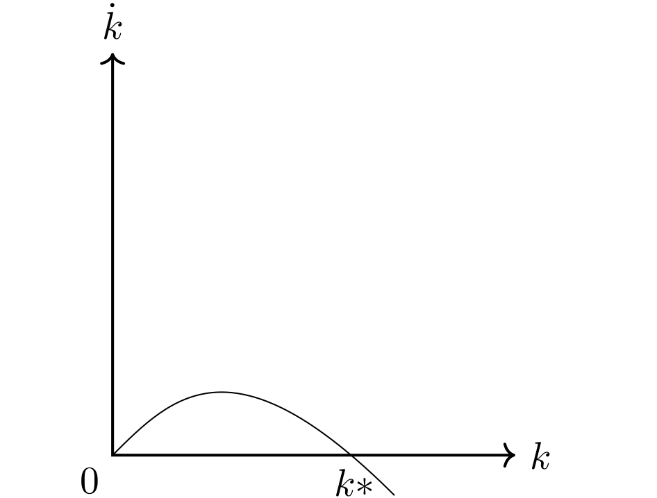
22.4.8 Steady-state \(k^*\)
The steady-state equilibrium capital, \(k^*\), is the point where: \[\dot{k} = 0.\] At this point, growth is zero as capital per effective labor unit \(k\) remains the same over time. Since output per effective unit of labor \(y\) depends on \(k\) through the production function, it is also unchanging. This point is described further in Table 22.1 and Figure 22.13.
| Variable | Symbol | Steady-state growth rate |
|---|---|---|
| Labor | \(L\) | \(n\) |
| Knowledge | \(A\) | \(g\) |
| Total output | \(Y = yAL\) | \(n+g\) |
| Capital per effective unit of labor | \(k = \frac{K}{AL}\) | 0 |
| Output per effective unit of labor | \(y = \frac{Y}{AL} = f(k)\) | 0 |
| Output per unit of labor | \(\frac{Y}{L} = yA\) | \(g\) |
22.4.9 Consumption
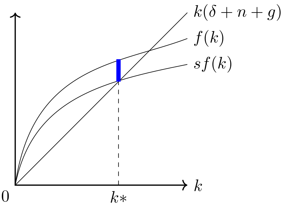
In the Solow model, \(sf(k)\) represents the proportion of output a country saves and invests. \(k(\delta + n+g)\) refers to the necessary investment to keep \(k\) stable. Thus, the thick blue line denotes the fraction of overall production, \(f(k)\), that goes to consumption, \(c\):
\[ c = f(k) - sf(k) \]
The dashed line represents the proportion that is reinvested. In the steady-state, actual investments equal break-even investment, \((n+g+\delta)k^*\). Therefore, steady-state consumption is given by:
\[ c^* = f(k^*) - (n+g+\delta)k^* \]
22.4.10 Golden rule of consumption
Increased investment in the capital stock can only boost growth until the steady state is reached. Thus, the question arises: How much should we invest in the capital stock? The only variable we should consider in the long run when deciding how much to invest from the output, \(sf(k)\), is consumption. The reason is that consumption, not output, defines welfare. Maximal steady-state consumption, \(C^{*}\), is given by:
\[ \frac{\partial C^*}{\partial s} = \underbrace{\left[ f'(k^*) - (n+g+\delta)\right]}_{\text{Golden Rule}}\frac{\partial k^*}{\partial s} \]
The golden rule states that consumption is maximized at the point when the slope of the output function, \(f(k)\), equals \(n+g+\delta\) as shown in the upper panel of Figure 22.13.
22.4.11 Long-run growth rates
In the steady state, there is a balanced growth path where all variables grow at a constant rate, as shown in Table 22.1. Sustained growth requires technological progress, evident because output per worker is only driven by \(g\).
22.5 Summary
- The steady-state equilibrium is the point where investment spending equals spending on depreciation, and the capital-output ratio remains constant; at this point, growth is zero.
- The Solow model provides a framework to understand the transition of economies over time.
- Less developed economies have lower capital-output ratios; with accumulating capital, they can experience catch-up growth.
- Investment is determined by the domestic savings ratio and by capital inflow from abroad.
- Investment in capital increases capital per worker and leads to growth.
- As the stock of capital rises, the extra output from an additional unit of capital falls; this characteristic is called diminishing returns.
- In the long run, growth requires technological progress, meaning output per worker is only driven by \(g\) (ideas).