17  Decision theory

Learning objectives:

Students will be able to:

• Distinguish different theories of decision making.
• Calculate the optimal decision under certainty, uncertainty, and under risk.
• Describe and use various criteria of decision making.
• Simplify complex decision making situations and use formal approaches of decision making to guide the decision making behavior of managers.

Required readings: Finne (1998)

Bonanno, G. (2017). Decision making. Accessed March 21, 2023. https://faculty.econ.ucdavis.edu/faculty/bonanno/DM_Book.html

Recommended readings: Bonanno (2017, sec. 3)

17.1 Payoff table

Every decision has consequences. While these consequences can be complex, economists often simplify decision analysis using the concept of utility. In this framework, anything positive is regarded as utility, and anything negative is viewed as disutility. Ultimately, these outcomes can be represented by a single value, which we will refer to as the “payoff.”

In this sense, decision-making becomes straightforward: we simply choose the alternative that provides the highest payoff. For example, if you know the weather will be sunny, you might choose to wear a T-shirt and shorts. On a cold day, however, you would opt for warmer clothing. But since the state of nature (the weather) is not completely certain, your decision involves some degree of risk, assuming you have some idea of the likelihood of sunshine or cold weather. If you have no information about the weather at all, your decision is made under uncertainty.

In the following, I introduce the payoff table as a tool to stylize a situation in which a decision must be made. Specifically, I will describe three modes of decision-making: under certainty, under uncertainty, and under risk.

A payoff table, also known as a decision matrix, can be a helpful tool for decision making, as shown in the table below. It presents the available alternatives denoted by $A_i$, along with the possible future states of nature denoted by $N_j$. A state of nature (or simply “state”) refers to the set of external factors (he has no direct power in it) that are relevant to the decision maker.

The payoff or outcome depends on both the chosen alternative and the future state of nature that occurs. For instance, if alternative $A_i$ is chosen and state of nature $N_j$ occurs, the resulting payoff is $O_{ij}$. Our goal is to choose the alternative $A_i$ that yields the most favorable outcome $O_{ij}$.

The payoff is a numerical value that represents either profit, cost, or more generally, utility (benefit) or disutility (loss).

Table 17.1: Payoff matrix

State of nature ($N_j$)	$N_1$	$N_2$	$\cdots$	$N_j$	$\cdots$	$N_n$
Probability (p)	$p_1$	$p_2$	$\cdots$	$p_j$	$\cdots$	$p_n$
Alternative ($A_i$)
$A_1$	$O_{11}$	$O_{12}$	$\cdots$	$O_{1j}$	$\cdots$	$O_{1n}$
$A_2$	$O_{21}$	$O_{22}$	$\cdots$	$O_{2j}$	$\cdots$	$O_{2n}$
$\cdots$	$\cdots$	$\cdots$	$\cdots$	$\cdots$	$\cdots$	$\cdots$
$A_i$	$O_{i1}$	$O_{i2}$	$\cdots$	$O_{ij}$	$\cdots$	$O_{in}$
$\cdots$	$\cdots$	$\cdots$	$\cdots$	$\cdots$	$\cdots$	$\cdots$
$A_m$	$O_{m1}$	$O_{m2}$	$\cdots$	$O_{mj}$	$\cdots$	$O_{mn}$

If we assume that all states are independent from each other and that we are certain about the state of nature, the decision is straightforward: just go for the alternative with the best outcome for each state of nature. However, most real-world scenarios are not that simple because most states of nature are more complex and needs further to be considered.

Decision making under uncertainty assumes that we are fully unaware of the future state of nature.

If a decision should be made under risks, then we have some information about the probability that certain states appear. A decision under uncertainty simple means we have no information, that is, no probabilities.

Warning

Unless stated otherwise, the outputs in a payoff table represent utility (or profits), where a higher number indicates a better outcome. However, the outputs could also represent something negative, such as disutility (or deficits). In such cases, the interpretation—and the decision-making process—changes significantly. Please keep this in mind.

17.2 Certainty

When a decision must be made under certainty, the state of nature is fully known, and the optimal choice is to select the alternative with the highest payoff. However, determining this payoff can be complex, as it may be the result of a sophisticated function involving multiple variables.

For example, imagine you need to choose between four different restaurants ($a_1$, $a_2$, $a_3$, $a_4$). Each restaurant offers a unique combination of characteristics, such as the quality of the food ($k_1$), the quality of the music played ($k_2$), the price ($k_3$), the quality of the service ($k_4$), and the overall environment ($k_5$). The corresponding payoff Table 17.2 assigns a numerical value to each characteristic, with higher numbers indicating better quality.

In this scenario, $a_i$ represents the different restaurant options, $k_i$ refers to specific characteristics of each restaurant, and the numbers in the table indicate the payoffs associated with each characteristic.

Please note that the characteristics $k_j$ of the scheme in Table 17.2 do not represent different states of nature but represent characteristics and its corresponding utility (whatever that number may mean in particular) of one particular characteristics if we choose a respective alternative.

Table 17.2: Weighting scheme

	$k_1$	$k_2$	$k_3$	$k_4$	$k_5$
$a_1$	3	0	7	1	4
$a_2$	4	1	4	2	1
$a_3$	4	0	3	2	1
$a_4$	5	1	2	3	1

Domination

To arrive at an overall outcome for each alternative and make an informed decision, the first step is to determine whether any alternatives are dominated by others. An alternative is considered dominated if it is not superior in any characteristic compared to at least one other alternative.

Dominated alternatives can be excluded from consideration. For example, in Table 17.3, we can see that alternative 2 outperforms alternative 3. This makes it unnecessary to consider alternative 3 in the decision-making process.

Table 17.3: Alternative 3 is dominated by alternative 2

	$k_1$	$k_2$	$k_3$	$k_4$	$k_5$
$a_1$	3	0	7	1	4
$a_2$	4	1	4	2	1
$a_3$	4	0	3	2	1
$a_4$	5	1	2	3	1

Weighting

No preferences

Still, we have three alternative left. How to decide? Well, we need to become clear what characteristics matter (most). Suppose you don’t have any preferences than you would go for restaurant $a_1$ because it offers the best average value, see Table 17.4.

Table 17.4: Alternative 1 is the best on average

	$k_1$	$k_2$	$k_3$	$k_4$	$k_5$	Overall
$a_1$	3	0	7	1	4	14/5
$a_2$	4	1	4	2	1	12/5
$a_4$	5	1	2	3	1	12/5

Clear preferences

Suppose you have a preference for the first three characteristics, that are quality of the food ($k_1$), the quality of the music played ($k_2$), and the price ($k_3$). Specifically, suppose that your preference scheme is as follows:

$$g_1:g_2:g_3:g_4:g_5=3:4:3:1:1$$

This means, for example, that you value music ($k_2$) four times more than the quality of the service ($k_4$) and the overall environment ($k_5$). The weights assigned to each characteristic are:

$$w_1=3/12;w_2=4/12;w_3=3/12;w_4=w_5=1/12.$$

To determine the best decision, you can calculate the aggregated expected utility for each alternative as follows:

$$\mathrm{\Phi }(a_i)=\sum _c{w}_p\cdot u_{ic}\to max,$$

where $u_{ic}$ represents the utility (or value) of alternative $i$ for a given characteristic $c$. The results of this calculation are shown in Table 17.5.

Table 17.5: Results with preferences given

	$k_1$	$k_2$	$k_3$	$k_4$	$k_5$	$\mathrm{\Phi }(a_i)$
$a_1$	3	0	7	1	4	35/12
$a_2$	4	1	4	2	1	31/12
$a_4$	5	1	2	3	1	29/12

Thus, alternative $a_1$ offers the best value given the preference scheme outlined above. In summary, we express the choice as follows: $$a_1\succ a_2\succ a_4\succ a_3,$$ where $\succ$ represents the preference relation (that is, “is preferred to”). If two alternatives offer the same value and we are indifferent between them, we can use the symbol $\sim$ to represent this indifference.

Maximax (go for cup)

If you like to go for cup, that is, you search for a great experience in at least one characteristic, then, you can choose the alternative that gives the maximum possible output in any characteristic. The choice would in our example be (see Table 17.6): $$a_1\succ a_4\succ a_2\sim a_3,$$

Table 17.6: Results with maximax

	$k_1$	$k_2$	$k_3$	$k_4$	$k_5$	Overall
$a_1$	3	0	7	1	4	7
$a_2$	4	1	4	2	1	4
$a_3$	4	0	3	2	1	4
$a_4$	5	1	2	3	1	5

Minimax (best of the worst)

The Minimax (or maximin) criterion is a conservative criterion because it is based on making the best out of the worst possible conditions. The choice would in our example be (see Table 17.7): $$a_2\sim a_4\succ a_1\sim a_3,$$

Table 17.7: Results with maximax

	$k_1$	$k_2$	$k_3$	$k_4$	$k_5$	Overall
$a_1$	3	0	7	1	4	0
$a_2$	4	1	4	2	1	1
$a_3$	4	0	3	2	1	0
$a_4$	5	1	2	3	1	1

Körth’s Maximin-Rule

According to this rule, we compare alternatives by the worst possible outcome under each alternative, and we should choose the one which maximizes the utility of the worst outcome. More concrete, the procedure consists of 4 steps:

1. Calculate the utility maximum for each column $c$ of the payoff matrix (see Table 17.8): $${\bar{O}}_c=\underset{i=1,\dots ,m}{max}{O}_{ic}\mathrm{\forall }c.$$

Table 17.8: Best utility per alternative

	$k_1$	$k_2$	$k_3$	$k_4$	$k_5$
$a_1$	3	0	7	1	4
$a_2$	4	1	4	2	1
$a_3$	4	0	3	2	1
$a_4$	5	1	2	3	1
${\bar{O}}_c$	5	1	7	3	4

2. Calculate for each cell the relative utility (see Table 17.9), $$\frac{O_{ij}}{{\bar{O}}_j}.$$

Table 17.9: Best relative utility

	$k_1$	$k_2$	$k_3$	$k_4$	$k_5$
$a_1$	3/5	0/1	7/7	1/3	4/4
$a_2$	4/5	1/1	4/7	2/3	1/4
$a_3$	4/5	0/1	3/7	2/3	1/4
$a_4$	5/5	1/1	2/7	3/3	1/4

3. Calculate for each row $i$ the minimum (see Table 17.10): $$\mathrm{\Phi }(a_i)=\underset{j=1,\dots ,p}{min}\left(\frac{O_{ij}}{{\bar{O}}_j}\right)\mathrm{\forall }i.$$

Table 17.10: Relative minimum for each alternative

	$k_1$	$k_2$	$k_3$	$k_4$	$k_5$	$\mathrm{\Phi }(a_i)$
$a_1$	3/5	0/1	7/7	1/3	4/4	0
$a_2$	4/5	1/1	4/7	2/3	1/4	1/4
$a_3$	4/5	0/1	3/7	2/3	1/4	0
$a_4$	5/5	1/1	2/7	3/3	1/4	1/4

4. Set preferences by maximizing $\mathrm{\Phi }(a_i)$: $$a_2\sim a_4\succ a_1\sim a_3,$$

Exercise 17.1 Körth

For the following payoff-matrix, calculate the order of preferences based on Körth’s Maximin-Rule.

$O_{ij}$	$k_1$	$k_2$	$k_3$	$k_4$	$k_5$
$a_1$	3	0	7	1	4
$a_2$	4	0	4	2	1
$a_3$	4	-1	3	2	1
$a_4$	5	1	3	3	1

Solution

${\bar{O}}_1=5;{\bar{O}}_2=1;{\bar{O}}_3=7;{\bar{O}}_4=3;{\bar{O}}_5=4$

$O_{ij}$	$k_1$	$k_2$	$k_3$	$k_4$	$k_5$	$\mathrm{\Phi }(a_i)$
$a_1$	3/5	0	1	1/3	1	0
$a_2$	4/5	0	4/7	2/3	1/4	0
$a_3$	4/5	-1	3/7	2/3	1/4	-1
$a_4$	1	1	3/7	1	1/4	1/4

$a_4\succ a_1\sim a_2\succ a_3$

Exercise 17.2 Given the following payoff table Table 17.11 where high numbers indicate high utility, ranging from $0$ (no utility) to $10$ (high utility).

Table 17.11: Payoff table

	z1	z2	z3	z4	z5
a1	1	2	3	4	3
a2	4	3	2	1	4
a3	4	5	0	5	6
a4	1	5	1	5	6
a5	2	2	2	1	3
a6	3	4	0	5	3

1. State which alternatives can be excluded because they are dominated by other alternatives.
   
2. Suppose your preference scheme is as follows: $$g_1=\frac{1}{2};g_2=1;g_3=2;g_4=1;g_5=1.$$ Find the order of preference based on the aggregated expected utility.

17.3 Uncertainty

When a decision must be made under uncertainty, the state of nature is fully unknown. That is, different possible states of nature exist but no information on their probability of occurrences are given. The optimal rational choice can’t be made without a criterion that reflect preferences such as risk aversion. In the following, I discuss some popular criteria.

Laplace criterion

The Laplace criterion assigns equal probabilities to all possible payoffs for each alternative, then selects the alternative with the highest expected payoff. An example can be found in Finne (1998). In Table 17.12 are the data for another example. According to the expected average utility, the decision should be $$a_2\succ a_1\succ a_3.$$

Table 17.12: Example data for uncertainty

Alternatives	$N_1$	$N_2$	$N_3$	Laplace	Maximax	Minimax
$a_1$	30	40	50	120/3	50	30
$a_2$	25	70	30	125/3	70	25
$a_3$	10	20	80	110/3	80	10

Maximax criterion (go for cup)

If you’re aiming for the best possible outcome without regard for the potential worst-case scenario, you would choose the alternative with the highest possible payoff. This “go for cup” approach focuses on maximizing the best-case outcome.

In the example of Table 17.12, the decision applying the Maximax strategy is $$a_3\succ a_2\succ a_1.$$

Minimax criterion (best of the worst)

The Minimax (or Maximin) criterion is a conservative approach, aimed at securing the best outcome under the worst possible conditions. This approach is often used by risk-averse decision-makers. For examples on how to apply this criterion, see Finne (1998).

In the example of Table 17.12, the decision applying the Maximax strategy is $$a_1\succ a_2\succ a_3.$$

Savage Minimax criterion

The Savage Minimax criterion minimizes the worst-case regret by selecting the option that performs as closely as possible to the optimal decision. Unlike the traditional minimax, this approach applies the minimax principle to the regret (that is, the difference or ratio of payoffs), making it less pessimistic. For more details, see Finne (1998).

Using the example data of Table 17.12, the regret table is constructed by subtracting the maximum payoff in each state from the payoffs in that state, see Table 17.13.

Table 17.13: Savage regret table

Alternatives	Regret for $N_1$	Regret for $N_2$	Regret for $N_3$	Maximum Regret
$a_1$	$30-30=0$	$70-40=30$	$80-50=30$	30
$a_2$	$30-25=5$	$70-70=0$	$80-30=50$	50
$a_3$	$30-10=20$	$70-20=50$	$80-80=0$	50

Based on the Savage Minimax criterion, the alternative with the smallest maximum regret should be chosen and the decision is $$a_1\succ a_2\sim a_3.$$

Hurwicz criterion

The Hurwicz criterion allows the decision-maker to calculate a weighted average between the best and worst possible payoff for each alternative. The alternative with the highest weighted average is then chosen.

For each decision alternative, the weight $\alpha$ is used to compute Hurwicz the value: $$H_i=\alpha \cdot {\bar{O}}_i+(1-\alpha )\cdot {\underset{―}{O}}_i$$ where $${\bar{O}}_i=\underset{j=1,\dots ,p}{max}{O}_{ij}\mathrm{\forall }i$$ and
$${\underset{―}{O}}_i=\underset{j=1,\dots ,p}{min}{O}_{ij}\mathrm{\forall }i,$$ that is, the respective maximum and minimum output for each alternative, $i$.

This formula allows for flexibility in decision-making by adjusting the value of $\alpha$, which reflects the decision-maker’s optimism (with $\alpha =1$ representing complete optimism and $\alpha =0$ representing complete pessimism).

The Hurwicz criterion calculates a weighted average between the best and worst payoffs for each alternative. Using the data of Table 17.12 once again, we need to assume an optimism index. Let’s say we are slightly optimistic and willing to take some risks by setting $\alpha =0.6$.

In $a_1$, the maximum payoff is 50 and the minimum payoff is 30. $$H_1=0.6\cdot 50+(1-0.6)\cdot 30=30+12=42$$

In $a_2$, the maximum payoff is 70 and the minimum payoff is 25. $$H_2=0.6\cdot 70+(1-0.6)\cdot 25=42+10=52$$

In $a_3$, the maximum payoff is 80 and the minimum payoff is 10. $$H_3=0.6\cdot 80+(1-0.6)\cdot 10=48+4=52$$

Thus, the decision is $$a_2\sim a_3\succ a_1.$$

Exercise 17.3 Use the data of Table 17.12 to make a decision for a complete pessimist ($\alpha =0$) and an optimist ($\alpha =1$)

Solution

When $\alpha =0$:

• $a_1$: ( H_1 = 30 )
• $a_2$: ( H_2 = 25 )
• $a_3$: ( H_3 = 10 )

Thus, the decision is $$a_1\succ a_2\succ a_3.$$

When $\alpha =1$:

• $a_1$: ( H_1 = 50 )
• $a_2$: ( H_2 = 70 )
• $a_3$: ( H_3 = 80 )

Thus, the decision is $$a_3\succ a_2\succ a_1.$$

Error in Finne (1998)

The example that is shown in Figure 7 of Finne (1998, p. 401) contains some errors. Here is the correct table including the Hurwicz-values (we assume a $\alpha =.5$):

$O_{ij}$	$min({\theta }_1)$	$max({\theta }_2)$	$H_i$
$a_1$	36	110	73
$a_2$	40	100	70
$a_3$	58	74	66
$a_4$	61	66	63.5

Thus, the order of preference is $a_4\succ a_3\succ a_1\succ a_2$.

Three categories

Read Finne (1998) and answer the following questions:

1. Explain the three categories of decision making.
2. Give examples of the three categories of decision making.
3. Explain the four criteria for decision making under uncertainty.

Finne, T. (1998). The three categories of decision-making and information security. Computers & Security, 17(5), 397–405.

Exercise 17.4  

Table 17.14: Payoff table

	z1	z2	z3
a1	0	9	8
a2	8	5	9
a3	1	10	1
a4	4	5	2
a5	9	10	10

In Table 17.14 you see a payoff table where high numbers indicate high disutility, ranging from $0$ (no disutility) to $10$ (high disutility).

1. Using this payoff table, indicate which alternatives can be excluded because they are dominated by other alternatives. (Hint: Exclude dominated alternatives in the calculations of the following questions).
   
2. Using the , calculate the complete order of preferred alternative(s), $a_i$.
3. Using the , calculate the complete order of preferred alternative(s), $a_i$.
4. Using the , calculate the complete order of preferred alternative(s), $a_i$.

17.4 Risk

When some information is given about the probability of occurrence of states of nature, we speak of decision-making under risk. The most straight forward technique to make a decision here is to maximize the expected outcome for each alternative given the probability of occurrence, $p_j$.

However, the expected utility hypothesis states that the subjective value associated with an individual’s gamble is the statistical expectation of that individual’s valuations of the outcomes of that gamble, where these valuations may differ from the Euro value of those outcomes. Thus, you should better look on the utility of a respective outcome rather than on the outcome itself because the utility and outcome do not have to be linked in a linear way. The St. Petersburg Paradox by Daniel Bernoulli in 1738 is considered the beginnings of the hypothesis.

Infinite St. Petersburg lotteries

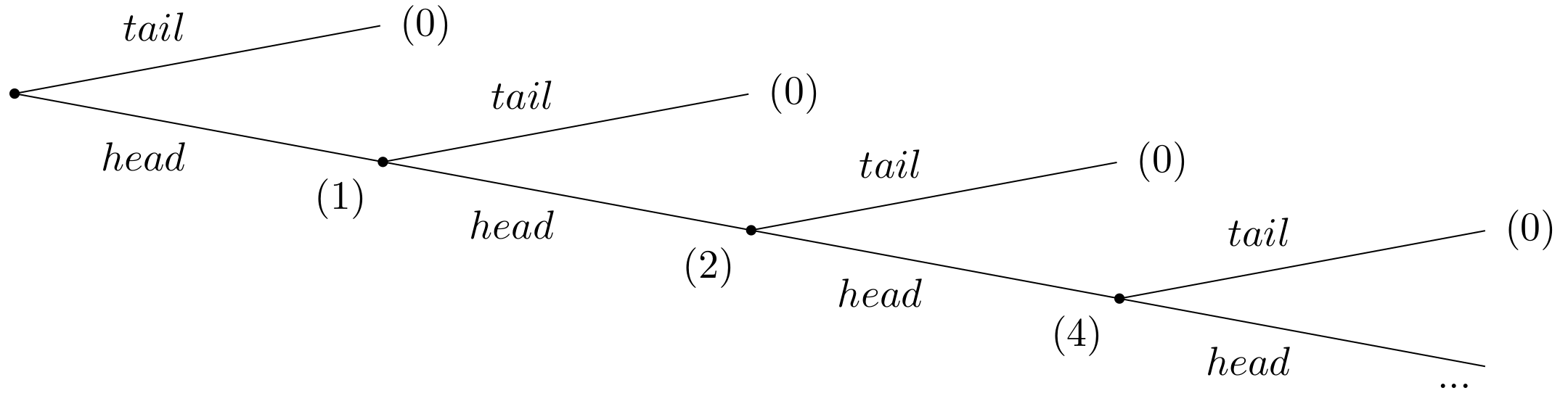
Suppose a casino offers a game of chance for a single player, where a fair coin is tossed at each stage. The first time head appears the player gets $1. From then onwards, every time a head appears, the stake is doubled. The game continues until the first tails appears, at which point the player receives $\mathrm{\$}{2}^{k-1}$, where k is the number of tosses (number of heads) plus one (for the final tails). For instance, if tails appears on the first toss, the player wins $0. If tails appears on the second toss, the player wins $2. If tails appears on the third toss, the player wins $4, and so on. The extensive form of the game is given in Figure 17.1.

Figure 17.1: Extensive form of the St. Petersburg paradox

Given the rules of the game, what would be a fair price for the player to pay the casino in order to enter the game?

To answer this question, one needs to consider the expected payout: The player has a 1/2 probability of winning $1, a 1/4 probability of winning $2, a 1/8 probability of winning $4, and so on. Thus, the overall expected value can be calculated as follows: $$E=\frac{1}{2}\cdot 1+\frac{1}{4}\cdot 2+\frac{1}{8}\cdot 4+\frac{1}{16}\cdot 8+\dots$$ This can be simplified as: $$E=\frac{1}{2}+\frac{1}{2}+\frac{1}{2}+\frac{1}{2}+\cdots =+\mathrm{\infty }.$$ That means the expected win for playing this game is an infinite amount of money. Based on the expected value, a risk-neutral individual should be willing to play the game at any price if given the opportunity. The willingness to pay of most people who have given the opportunity to play the game deviates dramatically from the objectively calculable expected payout of the lottery. This describes the apparent paradox.

In the context of the St. Petersburg Paradox, it becomes evident that relying solely on expected values is inadequate for certain games and for making well-informed decisions. Expected utility, on the other hand, has been the prevailing concept used to reconcile actual behavior with the notion of rationality thus far.

Finite St. Petersburg lotteries

Let us assume that at the beginning, the casino and the player agrees upon how many times the coin will be tossed. So we have a finite number I of lotteries with $1\le I\le \mathrm{\infty }$.

To calculate the expected value of the game, the probability $p(i)$ of throwing any number $i$ of consecutive head is crucial. This probability is given by $$p(i)=\underset{i\text{ factors}}{\underbrace{\frac{1}{2}\cdot \frac{1}{2}\cdot \cdots \frac{1}{2}}}=\frac{1}{2^i}$$ The payoff $W(I)$ is, if head appears $I$-times in a row by $$W(I)=2^{I-1}$$ The expected payoff $E(W(I))$ if the coin is flipped $I$ times is then given by $$E(W(I))=\sum _{i=1}^{I}p(i)\cdot W(i)=\sum _{i=1}^I\frac{1}{2^i}\cdot 2^{i-1}=\sum _{i=1}^I\frac{1}{2}=\frac{I}{2}$$

Thus, the expected payoff grows proportionally with the maximum number of rolls. This is because at any point in the game, the option to keep playing has a positive value no matter how many times head has appeared before. Thus, the expected value of the game is infinitely high for an unlimited number of tosses but not so for a limited number of tosses. Even with a very limited maximum number of tosses of, for example, $I=100$, only a few players would be willing to pay $50 for participation. The relatively high probability to leave the game with no or very low winnings leads in general to a subjective rather low evaluation that is below the expected value.

In the real world, we understand that money is limited and the casino offering this game also operates within a limited budget. Let’s assume, for example, that the casino’s maximum budget is $20,000,000. As a result, the game must conclude after 25 coin tosses because $2^{25}=33,554,432$ would exceed the casino’s financial capacity. Consequently, the expected value of the game in this scenario would be significantly reduced to just $12.50. Interestingly, if you were to ask people, most would still be willing to pay less than $12.50 to participate. How can we explain this? Well, it is not the expected outcome that matters but the utility that stems from the outcome.

The impact of output on utility matters

Daniel Bernoulli (1700 - 1782) worked on the paradox while being a professor in St. Petersburg. His solution builds on the conceptual separation of the expected payoff and its utility. He describes the basis of the paradox as follows:

``Until now scientists have usually rested their hypothesis on the assumption that all gains must be evaluated exclusively in terms of themselves, i.e., on the basis of their intrinsic qualities, and that these gains will always produce a utility directly proportionate to the gain.’’ (Bernoulli, 1954, p. 27)

Bernoulli, D. (1954). Exposition of a new theory on the measurement. Econometrica, 22(1), 23–36.

The relationship between gain and utility, however, is not simply directly proportional but rather more complex. Therefore, it is important to evaluate the game based on expected utility rather than just the expected payoff. $$E(u(W(I)))=\sum _{i=1}^{I}p(i)\cdot u(W(i))=\sum _{i=1}^I\frac{1}{2^i}\cdot u\left(2^{i-1}\right)$$ Daniel Bernoulli himself proposed the following logarithmic utility function: $$u(W)=a\cdot \ln (W),$$ where $a$ is a positive constant. Using this function in the expected utility, we get $$E(u(W(I)))=\sum _{i=1}^I\frac{1}{2^i}\cdot a\cdot \ln \left(2^{i-1}\right)=a\cdot \sum _{i=1}^I\frac{i-1}{2^i}\ln 2=a\cdot \ln 2\cdot \sum _{i=1}^I\frac{i-1}{2^i}.$$ The infinite series, $\sum _{i=1}^I\frac{i-1}{2^i}$, converges to 1 ($\underset{I\to \mathrm{\infty }}{lim}\sum _{i=1}^I\frac{i-1}{2^i}=1$). Thus, given an ex ante unbounded number of throws, the expected utility of the game is given by $$E(u(W(\mathrm{\infty })))=a\cdot \ln 2.$$

In experiments in which people were offered this game, their willingness to pay was roughly between 2 and 3 Euro. Thus, the suggests logarithmic utility function seems to be a pretty realistic specification. The main reason is mathematically that the increasing expected payoff has decreasing marginal utility and hence the utility function reflects the risk aversion of many people.

Exercise 17.5 Rationality and risk

There are 90 balls in an box. It is known that 30 of them are red, the remaining 60 are blue or green. An individual can choose between the following lotteries:

	Payoff	probability
Lottery 1	100 Euro if a red ball is drawn 0 Euro else	$p=\frac{1}{3}$
Lottery 2	100 Euro if a blue ball is drawn 0 Euro else	$0\le p\le \frac{2}{3}$

In a second variant it has the choice between the following lotteries:

	Payoff	probability
Lottery 3	100 Euro if a red or green ball is drawn or 0 Euro else	$\frac{1}{3}\le p\le 1$
Lottery 4	100 Euro if a blue or green ball is drawn or 0 Euro else	$p=\frac{2}{3}$

1. Which of the lotteries does the individual choose on the basis of expected values (risk neutral)?
2. Which of the lotteries does the individual choose on the basis of expected utility if the utility of a payoff of $x$ is given by $u(x)=x^2$?
3. Empirical studies, e.g. , show, however, that most individuals will usually choose lotteries 1 and 4. will. Discuss: Is this consistent with rational behavior?

Solution

Read the Wikipedia entry about the Ellsberg paradox (2024):

“In decision theory, the Ellsberg paradox (or Ellsberg’s paradox) is a paradox in which people’s decisions are inconsistent with subjective expected utility theory. John Maynard Keynes published a version of the paradox in 1921. Daniel Ellsberg popularized the paradox in his 1961 paper,”Risk, Ambiguity, and the Savage Axioms”. It is generally taken to be evidence of ambiguity aversion, in which a person tends to prefer choices with quantifiable risks over those with unknown, incalculable risks.

Ellsberg’s findings indicate that choices with an underlying level of risk are favored in instances where the likelihood of risk is clear, rather than instances in which the likelihood of risk is unknown. A decision-maker will overwhelmingly favor a choice with a transparent likelihood of risk, even in instances where the unknown alternative will likely produce greater utility. When offered choices with varying risk, people prefer choices with calculable risk, even when those choices have less utility.”

Ellsberg paradox. (2024). Wikipedia, The Free Encyclopedia. https://en.wikipedia.org/wiki/Ellsberg_paradox