26 IS-LM model

Students will be able to:

Understand the power of fiscal and monetary policy in a general equilibrium.
Describe how the IS-LM model explains the interaction of real goods markets and financial markets in balancing interest rates and total output in an economy.
Explain how investment acts as the key channel through which changes in real interest rates affect GDP in the short run.
Recognize how the government or central bank can increase aggregate demand to combat economic downturns and crises.

Required readings:
Blanchard & Johnson (2013, ch. 5).

26.1 Putting the IS and the LM relations together

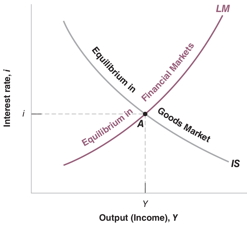
The IS relation stems from the condition that the supply of goods must equal the demand for goods, revealing how the interest rate affects output. Conversely, the LM relation stems from the condition that the supply of money must equal the demand for money, illustrating how output affects the interest rate. Now, by putting IS and LM relations together, we understand that at any time, both the supply of goods must equal the demand for goods, and the supply of money must equal the demand for money—both relations must hold. Together, they determine output and the interest rate.

The equilibrium in the goods market shows an interest rate increase leads to a decrease in output, depicted by the IS curve in Figure .

\[ \text{IS relation:} \quad C(Y-T) + I(Y,i) + G \]

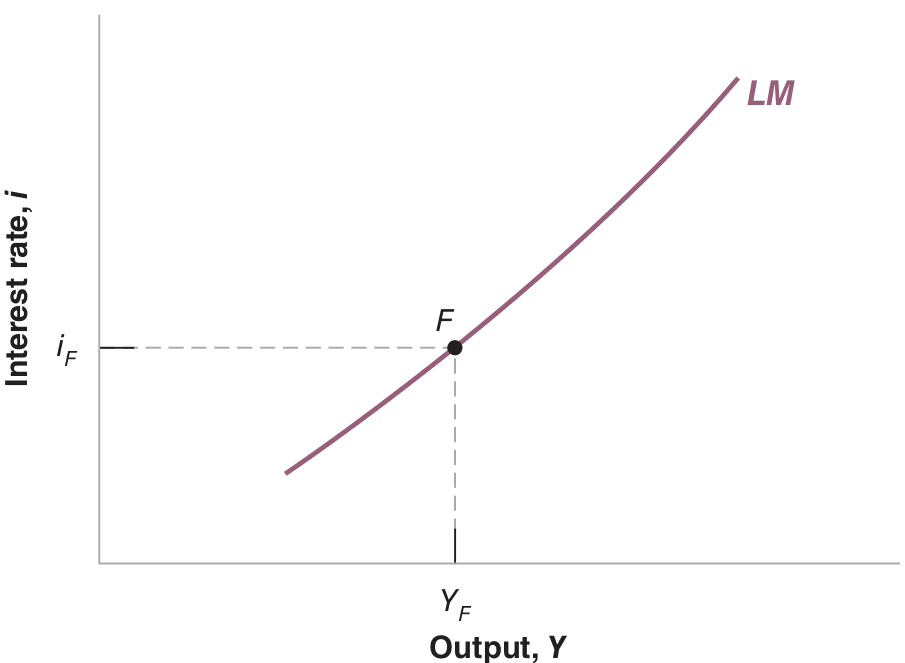
The equilibrium in financial markets implies an output increase leads to an interest rate increase, represented by the LM curve in Figure .

\[ \text{LM relation:} \quad \frac{M}{P} = YL(i) \]

The IS-LM model is visualized in Figure 26.1. Only at point A, where both curves intersect, are goods and financial markets in equilibrium.

You’ll notice the LM relation is expressed in real terms—relating real money (money in terms of goods), real income (income in terms of goods), and the interest rate. Remember: nominal GDP equals Real GDP times the GDP deflator: $\$Y = Y \cdot P$. Conversely, Real GDP equals nominal GDP divided by the GDP deflator: $\frac{\$Y}{P} = Y$.

26.2 Monetary policy

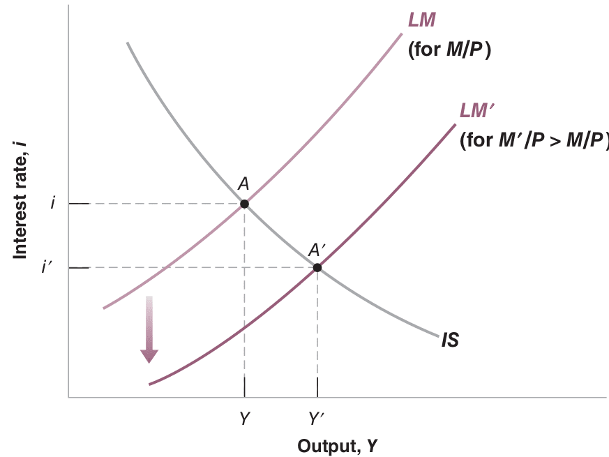
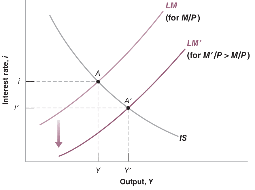
A monetary expansion results in higher output and lower interest rates. Conversely, the reverse holds for a monetary contraction. See Figure Figure 26.2.

Figure 26.2: The effects of a monetary expansion

26.2.0.1 Fiscal Policy

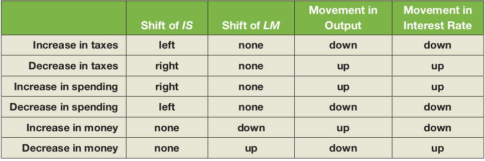
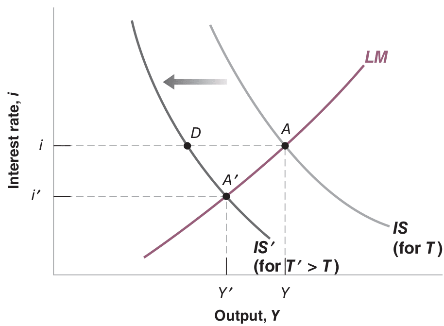
Fiscal contraction or consolidation refers to fiscal policy that reduces the budget deficit; increasing the deficit is called a fiscal expansion. Taxes and government spending affect the IS curve but not the LM curve, whereas changes in money supply impact the LM curve but not the IS curve. Figure 26.3 provides an overview of fiscal and monetary policy effects in the IS-LM model.

Figure 26.3: The effects of fiscal and monetary policy in the IS-LM model

Exercise 26.1 Fiscal contraction

What are the effects of this fiscal contraction on output, composition, and interest rates?
What are the effects of a monetary expansion?

Solution

When answering questions about the effects of policy changes, follow these three steps:

Equilibrium Impact:Determine how the change affects equilibrium in the goods market and the financial markets. Specifically, assess how it shifts the IS and/or the LM curves.
Intersection Effects: Characterize the effects of these shifts on the intersection of the IS and LM curves. Analyze what this does to equilibrium output and the equilibrium interest rate.
Descriptive Analysis: Describe the effects in words.

1. Impact on output:

Figure 26.4: Effects of fiscal contraction on output

Impact on financial markets:

Figure 26.5: Effects of fiscal contraction on financial markets

2. Overall Effects:

Figure 26.6: Overall effects of fiscal contraction

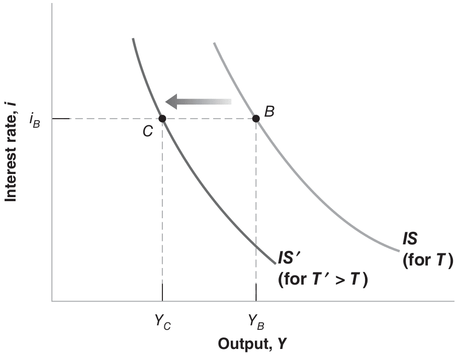
3. In Words: An increase in taxes leads to lower disposable income, causing people to reduce consumption. This decrease in demand, in turn, leads to a drop in output and income. Simultaneously, lower income reduces money demand, lowering the interest rate. The interest rate decline mitigates but does not fully counteract the increased tax impact on goods demand.

Effects of a Monetary Expansion

A monetary expansion results in higher output and a lower interest rate.

Figure 26.7: Effects of a monetary expansion

Blanchard, O., & Johnson, D. R. (2013). Macroeconomics (6th ed.). Pearson.

26.3 Limitations of the IS-LM model

It’s built on simplistic and unrealistic assumptions about the macroeconomy. Sir John Richard Hicks (1904-1989)¹ claimed the model’s flaws were fatal, better used as a “classroom gadget, to be superseded by something better.” However, new or optimized IS-LM frameworks have emerged over time.
The model’s a limited policy tool; it doesn’t detail how tax or spending policies should be formulated, limiting its practical appeal.
It lacks insights on inflation, rational expectations, or international markets, though later models attempt to incorporate these. The model also overlooks capital formation and labor productivity.

Hayek vs. Keynes

Friedrich August Hayek (1899-1992) opposed Keynesian policy, believing instead in the free market’s inherent price system to mitigate bust-and-boom cycles. In short, his view was that business cycles and economic crisis can only be avoided by trusting the free market and avoiding the boom itself. The clash between Keynesian and Classical/Austrian School economics is often represented with Keynes vs. Hayek analogies.

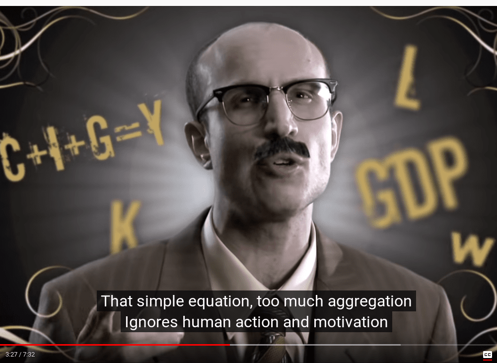
Exercise 26.2 Rap battle

Figure 26.8: Fear the Boom and Bust: Keynes vs. Hayek

Source: Youtube

Watch the video of Figure 26.8 and read the lyrics and comments at Genius Lyrics. Access comments on shaded text.

Explain the Keynesian strategy for combating bust and boom cycles. Explain Friedrich Hayek and the Austrian school’s approach to fighting bust-and-boom cycles. Also consider the video screenshots in Figure 26.9.

Solution

The Keynesian strategy focuses on government intervention to stabilize the economy using fiscal and monetary policies during recessions and expansions. Fiscal policies involve adjusting government spending and taxation, and monetary policies involve influencing interest rates and money supply.
Friedrich Hayek, unlike Keynes, advocated letting the market function freely without government or central bank manipulation, believing stable money supply and non-intervention to prevent cycles.

The Keynesian economic strategy for addressing bust and boom cycles hinges on government intervention to stabilize the economy, according to John Maynard Keynes. Bust and boom cycles—which encompass recessions and expansions—are seen as natural parts of the business cycle, potentially triggered by variations in consumer demand, credit availability, or government policy changes.

To counteract these cycles, Keynesian economists propose utilizing fiscal and monetary policies to stabilize the economy and foster growth. Fiscal policy involves modifying government spending and taxation to influence economic activity levels. For instance, during a recession, increased government spending on infrastructure or social welfare can boost demand and spur growth. Conversely, in an economic expansion, reducing spending or raising taxes can temper the economy and guard against overheating.

Monetary policy employs interest rate adjustments and money supply changes to influence economic activities. During a recession, the central bank might lower interest rates to encourage borrowing and investment, concurrently increasing the money supply by purchasing government bonds or other assets to stimulate demand and encourage growth. Conversely, during expansion phases, raising interest rates and decreasing money supply can help curb inflation and prevent overheating.

Overall, the Keynesian strategy employs a blend of fiscal and monetary policies to stabilize and spur economic growth.

Friedrich Hayek, an Austrian economist, preferred an approach distinct from Keynes’ to address bust and boom cycles. Hayek considered these cycles as stemming from money and credit manipulations by governments and central banks, with such interventions themselves fueling economic instability.

Hayek advocated for a free, non-interfered market system as the optimal means to address bust and boom cycles, discouraging fiscal or monetary manipulations by the government. He stressed allowing the market to self-regulate and adapt to shifting economic conditions.

He identified the business cycle as a result of “malinvestment,” occurring when money and credit supplies are artificially expanded, leading to unsustainable overinvestment in certain sectors. When credit expansions cease, these malinvestments become evident, sparking an economic downturn.

For Hayek, preventing bust and boom cycles required maintaining a stable, fixed money supply while dissuading the central bank from manipulating money and credit supplies. He also advised against government deficit spending or stimulating demand via increased spending, viewing such actions as catalysts for further instability and malinvestment.

In essence, Hayek’s approach to navigating bust and boom cycles pivoted on facilitating a free market without interference and stabilizing the money supply—a philosophy aligned with the Austrian School of economics.

Exercise 26.3 IS curve (0)

The following equations describe an economy:

\[ C = 10 + 0.5Y \] (Consumption function)

\[ I = 190 - 20i \] (Investment function)

\[ G = 0 \]

Derive the IS curve and represent it graphically.

Exercise 26.4 IS curve again

Given:

\[ \begin{aligned} C &= 100 + 0.75Y_d \\ I &= 50 - 25i \\ T &= G = 50 \end{aligned} \]

Where $C$ is consumption, $Y_d$ disposable income, $I$ investment, $T$ taxes, $G$ government purchases, $i$ interest rate. Derive the IS curve for the economy.

Exercise 26.5 IS curve (1)

Given behavioral equations:

\[\begin{align*} C &= 160 + 0.6Y_D \\ I &= 150 \\ G &= 150 \\ T &= 100 \end{align*}\]

Solve the following:

Equilibrium GDP ($Y$)
Disposable income ($Y_D$)
Consumption spending ($C$)

Exercise 26.6 IS curve (2)

Using the above economy:

Solve for equilibrium output. Compute total demand. Is it equal to production? Explain.
Assume $G$ is now 110. Solve for equilibrium output. Compute total demand. Is it equal to production? Explain.
Assume $G$ is 110, compute private plus public saving. Is it equal to investment? Explain.

Exercise 26.7 Automatic stabilizers

Assume fiscal policy variables $G$ and $T$ are independent of income. In reality, taxes depend on income and are higher when income’s high. Examine how automatic tax responses reduce autonomous spending impacts.

Behavioral equations:

\[\begin{align*} C &= c_0 + c_1Y_d \\ T &= t_0 + t_1Y \\ Y_d &= Y - T \end{align*}\]

$G$ and $I$ remain constant, $t_1$ is between 0 and 1.

Solve for equilibrium output.
What is the multiplier? Does the economy respond more to changes in autonomous spending when $t_1$ is 0 or positive? Explain.
Why is fiscal policy called an automatic stabilizer?

Exercise 26.8 IS-LM

Given the IS/LM model:

Consumption function: \[ C = 200 + 0.25(Y-T) \]

Investment function: \[ I = 150 + 0.25Y - 1000i \]

Fiscal policy: \[ G = 250 \] \[ T = 200 \]

Real money demand: \[ \left(\frac{M}{P}\right)^d = 2Y - 8000i \]

Real money supply: \[ \frac{M}{P} = 1600 \]

Answer these:

Derive the IS curve.
Derive the LM curve.
Solve for $Y^*$.
Solve for $i^*$.
Solve for $C^*$, $I^*$.
If $\frac{M}{P} = 1840$, repeat parts (a) through (e). Comment on equilibrium variable movement relative to initial $\frac{M}{P} = 1600$.
If $\frac{M}{P}=1600$, $G = 400$, repeat parts (a) through (e). Comment on equilibrium variable movement relative to initial $G = 250$.

Exercise 26.9 Foreign multiplier

Given macro aggregates for an economy:

\[ \begin{aligned} C &= 60 + 0.8Y_d \\ I &= 100 - 5i \\ i &= 0.06 \\ G &= 76 \\ T &= 15 \\ TR &= 60 \\ X &= 70 \\ M &= 12 + 0.2Y \end{aligned} \]

Where $TR$ denotes transfer payments, $X$ exports, $M$ imports. $TR$ affects disposable income $Y_d = Y - T + TR$.

Derive the IS curve using the data.
Calculate equilibrium income.
Calculate the foreign trade multplier and compare it with the multiplier when ignoring foreign trade. Interpret foreign trade’s impact on Keynesian policy.

British economist and major twentieth-century figure. See: John Hicks ↩︎