25 Financial market
Learning objectives:
Students will be able to:
- Understand the basic functioning of the money market.
- Recognize that money supply and money demand determine the interest rate.
- Explain how central banks influence money demand by influencing the interest rate.
- Analyze the effects of a monetary expansion.
- Derive the building blocks of our short-run model: the LM-curve.
Required readings:
Blanchard & Johnson (2013, ch. 5).
Recommended readings: Blanchard & Johnson (2013, ch. 4).
25.1 Semantic traps: Money, income, and wealth
Words such as money or wealth have specific meanings in economics, which differ from their everyday use.
25.1.0.1 Income
Income is what you earn from work plus what you receive in interest and dividends. It is a flow, meaning it is expressed per unit of time.
25.1.0.2 Saving
Saving is the part of after-tax income not spent, and it is also a flow. Savings is sometimes used as a synonym for wealth (a term we will not use here).
25.1.0.3 Financial wealth
Financial wealth, or simply wealth, is the value of all your financial assets minus liabilities. Unlike income or saving, financial wealth is a stock variable.
25.1.0.4 Investment
Investment is the purchase of new capital goods, like machines and buildings. Buying shares or financial assets is called financial investment.
25.1.0.5 Money
- can be used for transactions but pays no interest.
- two types of money:
- currency (coins and bills)
- checkable deposits (bank deposits on which you can write checks)
25.1.0.6 Bonds
Bonds pay a positive interest rate, \(i\), but cannot be used for transactions.
25.2 The demand for money
The demand for money comes from households, firms, and governments using money as a means of exchange and store of value. The law of demand holds: as the interest rate rises, the quantity of money demanded decreases because the interest rate represents an opportunity cost of holding money. Higher interest rates make money less effective as a store of value.
The demand for money depends on transactions in the economy and the interest rate. While transactions are hard to measure, they’re likely roughly proportional to nominal income. Demand for money is described as follows:
\[ M^d = \$Y \underbrace{L(i)}_{\frac{\partial L(i)}{\partial i} < 0} \]
Read this as: The demand for money \(M^d\) equals nominal income $Y times a function of the interest rate \(i\), denoted by \(L(i)\). An increase in the interest rate decreases money demand as people shift more wealth to bonds.
For a given nominal income, lower interest rates increase money demand. At a given interest rate, rising nominal income shifts money demand right. See Figure 25.1.
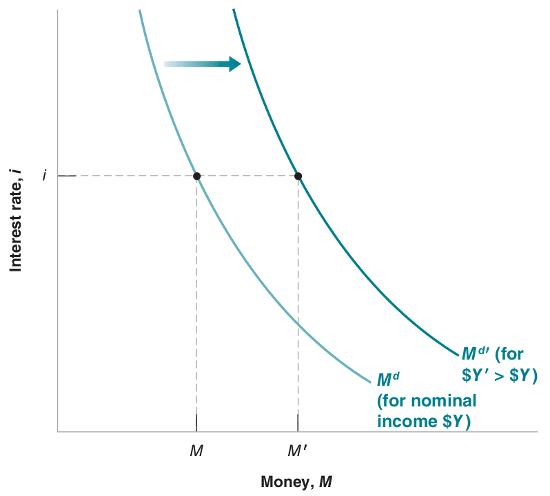
Note: Blanchard & Johnson (2013, p. 66)
25.3 The supply of money and equilibrium
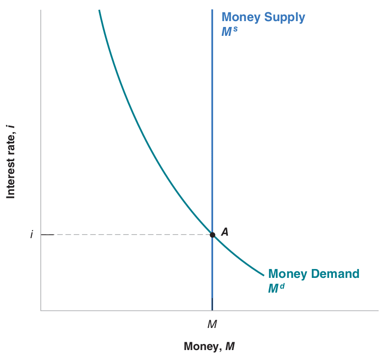
To find equilibrium in financial markets, understand that the price of money is the interest rate. Like any market, equilibrium is where demand and supply meet. Simplifying, assume monetary authorities (central banks) supply money and set interest rates.
A central bank can either choose money supply, setting interest rates where supply equals demand, or choose the interest rate and adjust money supply to achieve its chosen rate.
Equilibrium requires money supply equals money demand, \(M = M^d\):
\[ \underbrace{M}_{\text{money supply}} = \underbrace{\$Y L(i)}_{\text{money demand}} \]
This equilibrium relation is called the LM relation where LM stands for Liquidity and Money.1
Note: Blanchard & Johnson (2013, p. 68)
- The interest rate must be such that money supply (independent of interest rate) equals money demand (dependent on interest rate). See Figure Figure 25.2.
- An increase in nominal income raises the interest rate as shown in Figure Figure 25.3.
- As mentioned, a central bank lowering interest rates from \(i\) to \(i'\) is akin to increasing money supply, seen in Figure Figure 25.5.
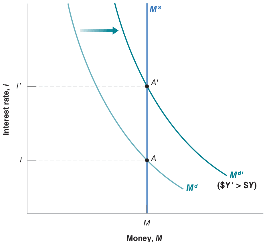
Note: Blanchard & Johnson (2013, p. 69)
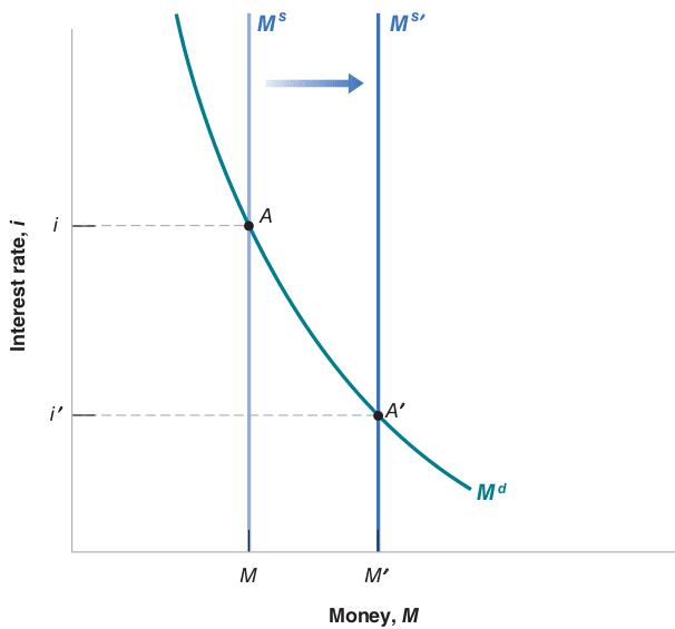
Note: Blanchard & Johnson (2013, p. 70)
25.4 The derivation of the LM curve
25.4.1 Using algebra
Assuming money demand is linear:
\[ M^d = Y - hi \quad \text{with } h > 0 \]
The parameter \(h\) represents how much demand for real money balances decreases as interest rates rise. Money supply (\(M\)) is set by the central bank and is assumed constant for a period. Solving for the interest rate gives the LM curve:
\[ i = \frac{1}{h} \left(Y - M\right) \]
25.4.2 Using graphs (see Figure 25.5)
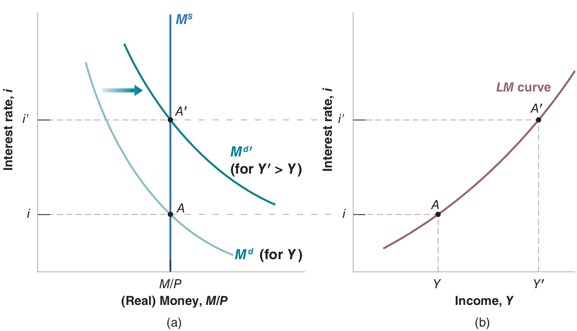
Note: Blanchard & Johnson (2013, p. 87)
- An income increase, at a given interest rate, raises demand for money. Given supply, this demand rise increases the equilibrium interest rate.
- Equilibrium in financial markets implies an income increase raises interest rates. The LM curve is upward sloping.
25.5 Taylor rule
- The Taylor rule derives from empirical insights into how central banks operate.
- It can replace the LM curve in the IS-LM Model, forming the IS-TR Model.
- It’s a formula predicting central banks’ interest rate changes due to economic shifts.
- The Taylor rule recommends raising interest rates when inflation or GDP growth exceed desired levels.
- Critics say the Taylor principle can’t account for sudden economic shocks.
- For more on the Taylor rule, see the Wikipedia entry: Taylor rule.
- Formally, the rule is expressed as:
\[ i_{t} = \pi_{t} + r_{t}^{*} + a_{\pi}(\pi_{t} - \pi_{t}^{*}) + a_{y}(y_{t} - \bar{y}_{t}) \]
In this equation:
- \(i_t\): target short-term nominal interest rate,
- \(\pi_{t}\): inflation rate per GDP deflator,
- \(\pi _{t}^{*}\): desired inflation rate (target inflation rate),
- \(r_{t}^{*}\): assumed equilibrium real interest rate,
- \(y_{t}\): logarithm of real GDP,
- \(\bar{y}_{t}\): logarithm of potential output (linear trend).
Empirics showed it looks like this for central banks like the ECB and FED:
\[ i_{t} = \pi _{t} + 2 + 0.5(\pi _{t} - 2\%) + 0.5(y_{t} - {\bar y}_{t}) \]
Economists use liquidity as a measure of how easily an asset can be exchanged for money. Money is fully liquid; other assets less so.↩︎